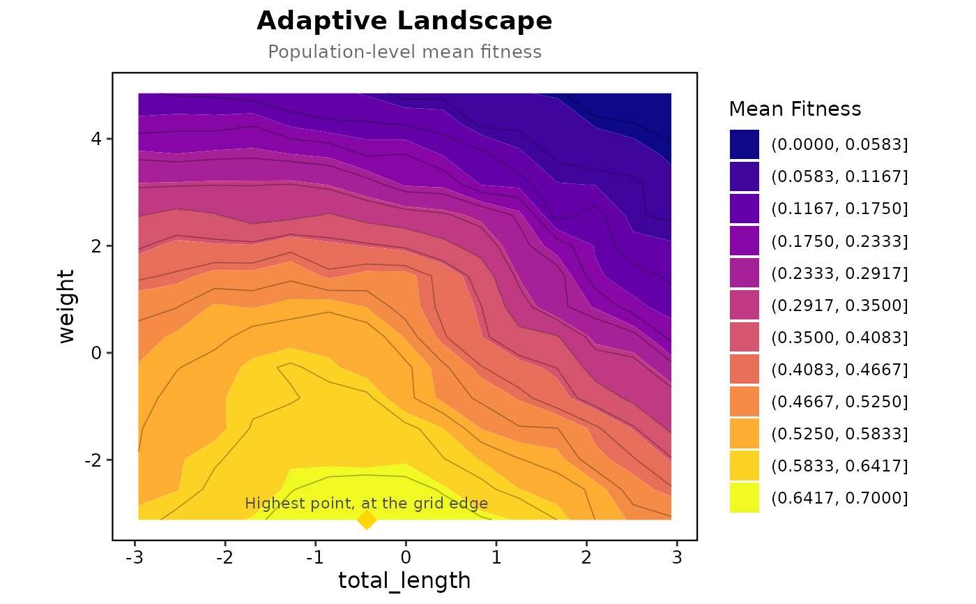
Plot Adaptive Landscape — plot_adaptive

Two traits give a contour map of mean fitness against the two population means. One trait gives a curve of mean fitness against the population mean, with the individual fitness function drawn alongside it for comparison.

Usage

plot_adaptive_landscape(
  landscape,
  trait_cols,
  original_data = NULL,
  group_col = NULL,
  bins = 12,
  show_optimum = TRUE,
  show_actual_means = TRUE,
  show_individual = TRUE,
  point_alpha = 0.8,
  show_support = FALSE,
  support_level = 0.5,
  ...
)

Arguments

landscape: Output object of class "adaptive_landscape".
trait_cols: One or two trait column names, matching the landscape.
original_data: Optional data frame of original data points. Default is NULL.
group_col: Optional character string specifying a grouping variable for labels.
bins: Integer specifying the number of contour bins. Default is 12.
show_optimum: Logical indicating whether to display the optimum point, labelled as the highest point when it lies on the edge of the grid. Default is TRUE.
show_actual_means: Logical indicating whether to display actual population means. Default is TRUE.
show_individual: Logical; for a single trait, also draw the individual fitness function (dashed). Default is TRUE.
point_alpha: Numeric value for point transparency. Default is 0.8.
show_support: Logical; mark where the simulation leaves the data: a dashed line at support_level and a white overlay on the population means beyond it, where more than that share of the simulated population falls outside the observed traits. Default is FALSE.
support_level: Share of the simulated population outside the data at which show_support draws its line. Default is 0.5.
...: Additional arguments passed to ggplot2::labs().

Value

A ggplot object representing the adaptive landscape.

Examples

prep <- prepare_selection_data(bumpus, "survival", c("total_length", "weight"))
surf <- correlated_fitness_surface(prep, "survival", c("total_length", "weight"), grid_n = 30)
#> Data type: binary; method: gam; n = 136; k = 29
#> GAM fitting with 136 observations
#>   Trying formula: main
#> Success with formula: main
#> Predictions range: 0.0472 to 0.703
#> Masked 424 of 900 grid points outside the data
land <- adaptive_landscape(prep, surf$model, c("total_length", "weight"),
                           simulation_n = 100, grid_n = 15)
#> Population mean grid ranges:
#>   total_length: -2.96 to 2.94
#>   weight: -3.12 to 4.85
#> Estimated within-population variance-covariance:
#>              total_length weight
#> total_length       1.0000 0.5839
#> weight             0.5839 1.0000
#> Calculating mean fitness for 225 grid points
#> Optimal population mean phenotype:
#>   total_length    weight
#> 7   -0.4336396 -3.121579
#> Mean fitness at optimum: 0.6814
#> The highest mean fitness is on the edge of the grid; the landscape may keep rising beyond it
#> 75% of simulated individuals fell outside the data (97% at the optimum)
#> The optimum rests on extrapolation: more than 25% of the population simulated there lies outside the data
plot_adaptive_landscape(land, c("total_length", "weight"))