Evolutionary Selection Analysis

A guide to the package, with worked examples

2026-07-13

Evolutionary Selection Analysis Framework

1. Overview

This package measures natural selection on phenotypic traits the way Lande & Arnold (1983) set out, and adds spline fitness functions, fitness surfaces and adaptive landscapes on top of the same prepared data. Svensson (2023) reviews the approach and the arguments about it; Palacio et al. (2019) set out what an analysis should report, and check_selection_assumptions() runs the checks they ask for on the data and the models.

Key capabilities:

Analysis Type	Description
Selection differentials ($\mathbf{S}$)	Total selection acting on traits
Linear selection gradients ($\boldsymbol{\beta}$)	Direct directional selection
Nonlinear selection gradients ($\boldsymbol{\gamma}$)	Stabilising/disruptive and correlational selection
Univariate correlated fitness functions	Flexible spline-based fitness functions at the individual level
Bivariate correlated fitness surfaces	Thin-plate spline (TPS) or GAM surfaces of individual fitness as a function of two traits
Adaptive landscapes	Mean fitness as a function of population mean phenotype (requires simulation)
Landscapes over time	One fitness function or surface per period, on trait axes shared by all periods
Canonical analysis	$\boldsymbol{\gamma}$ rotated to its canonical axes, and the curvature along each axis tested
Peak comparison	The difference in fitted fitness between two peaks, or between a peak and the valley between them, with its standard error
Uncertainty	Bootstrap intervals for the gradients; standard error lines or bands on GAM surfaces
Binary and count fitness	Logistic regression for survival; Poisson or negative binomial regression for offspring counts (p-values only; the gradients stay OLS)

---

2. Mathematical Framework

2.1 Relative Fitness

Individual fitness is converted to relative fitness to enable comparisons across populations and generations:

$$w_i = \frac{W_i}{\bar{W}}$$

where $W_i$ is the absolute fitness of individual $i$ (an offspring count, or survival coded 0/1), $\bar{W} = \frac{1}{n}\sum_{i=1}^n W_i$ is the mean fitness of the population, and $w_i$ is the relative fitness of individual $i$.

Fitness is made relative because selection acts on differences in fitness relative to the mean, and dividing by mean fitness puts gradients from different studies on one scale. Brodie and Janzen (1996) showed that regressing absolute survival puts the gradients on the wrong scale, which is why the package always relativises fitness before fitting. File: prepare_selection_data.R

2.2 Trait Standardisation

Traits are standardised to mean 0 and variance 1 before analysis:

$$z_i = \frac{x_i - \bar{x}}{s_x}$$

where $x_i$ is the original trait value, $\bar{x}$ and $s_x$ are the sample mean and standard deviation, and $z_i$ is the standardised value.

Purpose: Standardisation puts all traits on the same scale, allowing direct comparison of selection gradients. A $\beta = 0.5$ means that a one-standard-deviation increase in the trait increases relative fitness by 0.5 units.

Scale traits and relative fitness within the population and time period in question. With data from several years or sites, pass the column to group and both steps are done separately within each level before the data are stacked. For the linear gradients scaling within groups is the same as fitting a fixed effect for the group, and for the quadratic ones close to it, so the pooled gradients gain power from the extra individuals without mixing the groups’ scales, but the pooled model cannot test whether selection differs between groups (a year by trait interaction); fit the groups separately with return_grouped = TRUE for that.

The gradients are the raw partial regression coefficients from models fitted to these standardised traits, so don’t wrap the traits in scale() in a model formula or use a modelling option that standardises predictors; either would scale the coefficients a second time. File: prepare_selection_data.R

2.3 Selection Differential

The selection differential ($S$) measures the total selection acting on a trait, including both direct and indirect effects through correlated traits:

$$S = \text{Cov}(z, w) = \mathbb{E}[(z - \bar{z})(w - \bar{w})]$$

For multiple traits, the vector of selection differentials is:

$$\mathbf{S} = \text{Cov}(\mathbf{z}, w) = \begin{bmatrix} \text{Cov}(z_1, w) \\ \text{Cov}(z_2, w) \\ \vdots \\ \text{Cov}(z_m, w) \end{bmatrix}$$

It is the change in the trait mean within a generation (Arnold & Wade, 1984).

Interpretation: $S$ represents the shift in trait mean after one generation of selection. A positive $S$ indicates the trait mean increases. File: selection_differential.R

2.4 Linear Selection Gradients

Linear selection gradients ($\boldsymbol{\beta}$) measure the direct directional selection on each trait, controlling for correlations with other traits:

$$w = \alpha + \boldsymbol{\beta}^T \mathbf{z} + \varepsilon$$

In matrix form:

$$\boldsymbol{\beta} = \mathbf{P}^{-1} \mathbf{S}$$

where $\mathbf{P}$ is the phenotypic variance-covariance matrix.

For a model with two traits:

$$w = \alpha + \beta_1 z_1 + \beta_2 z_2 + \varepsilon$$

Interpretation: $\beta_i$ is the partial regression coefficient: the change in relative fitness for a one-standard-deviation increase in trait $i$, holding all other traits constant.

Tests. The gradients always come from this least-squares fit on relative fitness. Its t-tests are only valid when the residuals are roughly normal, which holds for continuous fitness but not for survival or offspring counts. For binary fitness the p-values therefore come from a logistic regression of the raw 0/1 outcome on the same terms, and for counts from a Poisson regression of the raw counts, replaced by a negative binomial one when the counts are overdispersed. File: analyze_linear_selection.R

2.5 Nonlinear Selection Gradients

Quadratic selection gradients ($\boldsymbol{\gamma}$) measure nonlinear selection, including stabilising/disruptive selection (diagonal elements) and correlational selection (off-diagonal elements):

$$w = \alpha + \boldsymbol{\beta}^T \mathbf{z} + \frac{1}{2} \mathbf{z}^T \boldsymbol{\gamma} \mathbf{z} + \varepsilon$$

For two traits, this expands to:

$$w = \alpha + \beta_1 z_1 + \beta_2 z_2 + \frac{1}{2}\gamma_{11} z_1^2 + \frac{1}{2}\gamma_{22} z_2^2 + \gamma_{12} z_1 z_2 + \varepsilon$$

Important: The $\frac{1}{2}$ factor in the quadratic terms follows Lande & Arnold’s convention, making $\gamma_{ii}$ the second derivative of the fitness surface. In practice, most implementations (including this one) report $2 \times$ the quadratic coefficient from regression, which equals $\gamma_{ii}$.

Interpretation:

$\gamma$ value	Type	Interpretation
$\gamma_{ii} < 0$	Stabilising selection	Intermediate trait values have highest fitness
$\gamma_{ii} > 0$	Disruptive selection	Extreme trait values have highest fitness
$\gamma_{ij} > 0$	Positive correlational	Selection favours positive correlation between traits
$\gamma_{ij} < 0$	Negative correlational	Selection favours negative correlation between traits

Canonical axes: with several traits the curvature is spread over the $\gamma_{ii}$ and the $\gamma_{ij}$ together. Canonical analysis (Phillips & Arnold, 1989; Blows & Brooks, 2003) rotates $\boldsymbol{\gamma}$ to its eigenvectors, combinations of the traits that each have a single curvature, the eigenvalue $\lambda$. See canonical_analysis() in section 5.17.

File: analyze_nonlinear_selection.R, analyze_disruptive_selection.R

2.6 Nonparametric Fitness Functions and Surfaces

Quadratic regression fixes the shape of the fitness function in advance, while a spline takes its shape from the data and can show, for example, two peaks that a quadratic would average away. These are still individual-level fitness functions; the population-level adaptive landscape is a separate construction (section 2.7). Cubic splines for one trait and thin-plate splines for two follow Schluter (1988) and Schluter and Nychka (1994); Brodie et al. (1995) is the guide to reading the surfaces.

Univariate spline model:

$$w = \alpha + s(z) + \varepsilon$$

where $s(z)$ is a smooth function estimated from the data using penalised regression splines.

Multivariate thin-plate spline:

$$w = \alpha + f(z_1, z_2) + \varepsilon$$

where $f(z_1, z_2)$ is a two-dimensional smooth surface showing how individual fitness varies across trait combinations. The univariate spline chooses its smoothing parameter by generalised cross-validation (Schluter 1988), which for survival and Poisson counts mgcv applies in its UBRE form; the surface uses REML. The surface is drawn only where there are data: grid points outside the convex hull of the observed trait pairs are blank, and a distance rule can also blank cells far from any individual, as Beausoleil et al. (2023) did for a community of Darwin’s finches. With a grouping column such as species, each group’s mean and the highest point of the surface within that group’s own range are marked on the plot.

GAM formulation: $$w \sim \text{family}(\eta), \quad \eta = \alpha + s(z_1, z_2)$$

File: correlated_fitness_surface.R

2.7 Adaptive Landscapes (Population Level)

Following Sewall Wright’s original concept, the adaptive landscape describes mean fitness as a function of population mean phenotype:

$$\bar{W} = g(\bar{z}_1, \bar{z}_2)$$

where:

• $\bar{W}$ = mean fitness of the population
  
• $\bar{z}_1, \bar{z}_2$ = population mean phenotypes

A fitness surface is fitted to individuals. The adaptive landscape is the mean fitness a population would have at a given mean phenotype, so it is computed by simulating such populations.

Calculation procedure:

For each candidate population mean $\bar{\mathbf{z}}$:

1. Simulate individuals around the mean

$$\mathbf{z}_{\text{ind}} \sim \mathrm{N}(\bar{\mathbf{z}}, \mathbf{P})$$

where $\mathbf{P}$ is the within-population phenotypic variance–covariance matrix.

2. Predict individual fitness

$$w_{\text{ind}} = \hat{f}(\mathbf{z}_{\text{ind}})$$

3. Compute mean fitness

$$\bar{W}(\bar{\mathbf{z}}) = \frac{1}{N_{\text{sim}}} \sum_{j=1}^{N_{\text{sim}}} w_{\text{ind}, j}$$

The resulting surface:

$$\bar{W} = g(\bar{z}_1, \bar{z}_2)$$

is the adaptive landscape.

Mathematical distinction

Surface	Level	Formula	Interpretation
Correlated Fitness	Individual	$w = f(\mathbf{z})$	Selection acting on individuals now
Adaptive Landscape	Population	$\bar{W} = g(\bar{\mathbf{z}})$	Where selection would move the population mean

File: adaptive_landscape.R

The two surfaces are compared with compare_fitness_surfaces_data() (section 5.15). The same construction works for a single trait, where the landscape is a curve of mean fitness against the population mean, drawn alongside the fitness function it was averaged from.

---

2.8 Landscapes over Time

Beausoleil et al. (2019) fitted a separate fitness function to each year of the finch data and found disruptive selection throughout, stronger in some years than others and significant in three of the six year-to-year intervals they tested. The package does the same with temporal_landscape(): the fitness function (one trait) or surface (two traits) and, if asked, the adaptive landscape are fitted separately for each level of a time column, on traits standardised once over all periods so that the periods share one axis. The result is one row per period with the sample size, mean fitness, the degrees of freedom of the smooth, the position of the highest fitness and, for one trait, the number of interior peaks. plot_temporal_landscape() draws the periods side by side or, for one trait, as a heat map of fitness against trait and time.

File: temporal_landscape.R

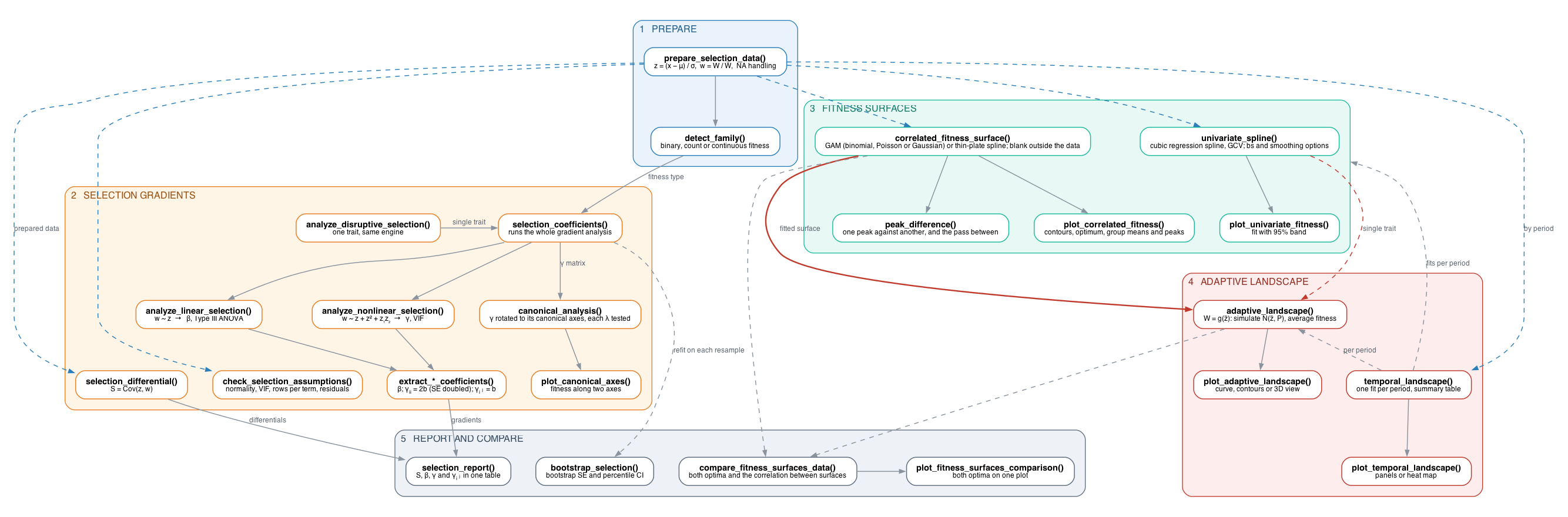
3. Framework Structure

3.1 Core Scripts and Their Roles

Script	Purpose	Key Functions	Mathematical Component
prepare_selection_data.R	Data preprocessing	Standardisation, relative fitness, NA handling	$z_i = \frac{x_i - \bar{x}}{s_x}$, $w_i = \frac{W_i}{\bar{W}}$
detect_family.R	Fitness type detection	Binary, count or continuous	$W_i \in \{0,1\}$, $W_i \in \mathbb{N}$ or $W_i \in \mathbb{R}^+$
selection_differential.R	Selection differential	$S = \text{Cov}(z, w)$	$S = \mathbb{E}[(z - \bar{z})(w - \bar{w})]$
selection_coefficients.R	Main wrapper	Complete analysis	Gradient estimation
analyze_linear_selection.R	Linear gradients	Regression	$w = \alpha + \boldsymbol{\beta}^T \mathbf{z} + \varepsilon$
analyze_nonlinear_selection.R	Quadratic gradients	$z^2$ + interactions	$w = \alpha + \boldsymbol{\beta}^T\mathbf{z} + \frac{1}{2}\mathbf{z}^T\boldsymbol{\gamma}\mathbf{z} + \varepsilon$
analyze_disruptive_selection.R	Single-trait quadratic	Stabilising/disruptive test	$\gamma_{ii} = 2\beta_{ii}$
extract_results.R	Result extraction	Coefficient parsing	$\beta$, $\gamma$
univariate_spline.R	1D fitness	Cubic regression spline (GCV, UBRE for 0/1 and Poisson counts)	$w = \alpha + s(z) + \varepsilon$
correlated_fitness_surface.R	2D fitness	GAM / TPS	$w = \alpha + f(z_1, z_2) + \varepsilon$
adaptive_landscape.R	Adaptive landscape	Simulation	$\bar{W} = g(\bar{z}_1, \bar{z}_2)$
compare_fitness_surfaces.R	Comparison	Surface contrast	Individual vs population
plot_correlated_fitness.R	Visualisation	Contour plots	2D fitness
plot_univariate_fitness.R	Visualisation	Line + 95% band	Wald interval or bootstrap ribbon
plot_adaptive_landscape.R	Visualisation	Population surface	$\bar{W}(\bar{z})$
temporal_landscape.R	Selection over time	One fit per period, summary table	$w_t = \alpha_t + s_t(z)$
plot_temporal_landscape.R	Visualisation	Panels or heat map by period	$w_t(z)$
selection_report.R	Results table	$S$, $\beta$, $\gamma$, $\gamma_{ij}$ together	Same individuals, same scale
bootstrap_selection.R	Uncertainty	Resampling with replacement	Bootstrap SE, percentile CI
check_selection_assumptions.R	Assumption checks	Normality, VIF, rows per term, residuals	Mardia’s tests, Shapiro-Wilk, Breusch-Pagan
canonical_analysis.R	Canonical analysis	Eigen-decomposition of $\boldsymbol{\gamma}$, double regression, permutation test	$\boldsymbol{\gamma} = \mathbf{M}\boldsymbol{\Lambda}\mathbf{M}^T$
peak_difference.R	Peak comparison	Difference in fitted fitness between two points, and between each and the pass between them	Link-scale difference, SE from the model’s covariance
run_app.R	Interactive app	The whole workflow in a browser	Same calculations as the functions above

3.2 Function Dependencies

Function dependencies. Drawn from workflow.dot with Graphviz.

Solid arrows show data passed from one function to the next. Blue dashed arrows carry the prepared data to the functions that use it directly; grey dashed arrows show a result being reused elsewhere.

---

4. Installation and Requirements

4.1 Loading the package

The package loads everything it needs:

library(lande)

4.2 Package Descriptions

mgcv, MASS, Matrix, ggplot2 and dplyr install with the package; the rest are needed only for the features listed.

Package	Purpose
mgcv	Generalised additive models (GAMs) for flexible spline-based fitness estimation
fields	Thin-plate spline (TPS) interpolation for bivariate fitness surfaces
MASS	Multivariate normal simulation (mvrnorm) for adaptive landscape generation
Matrix	Matrix operations and positive-definite corrections (nearPD)
car	Type III ANOVA and variance inflation factor (VIF) diagnostics
ggplot2	Visualisation of fitness functions and contour surfaces
dplyr	Data manipulation and transformation (filtering, summarising)
ggrepel	Improved text labelling in plots (avoids overlap)
viridis	Perceptually uniform colour scales for scientific visualisation
patchwork	Composing multiple plots into a single figure
performance	Heteroscedasticity, overdispersion and $R^2$ in the assumption checks
akima	Putting the two surfaces on one grid to correlate them in compare_fitness_surfaces_data()
shiny	The app, run_app()
plotly	The rotatable 3D landscape in the app

4.3 Example data and the app

Five datasets come with the package, each with a help page giving its columns and source: bumpus, the house sparrows of Bumpus (1899); crescent_pond_pupfish and little_lake_pupfish, the pupfish of Martin (2016); finch_yearly, the medium ground finches of Beausoleil et al. (2019); and finch_community, the five finch groups of Beausoleil et al. (2023). Most examples below use simulated data; sections 5.16, 5.17 and 7.0 use finch_yearly and bumpus.

run_app() runs the same workflow in a browser, on four of these datasets (all but finch_yearly) or an uploaded CSV, and writes out the R calls that repeat the analysis with its settings.

---

5. Detailed Function Reference

5.1 prepare_selection_data()

Purpose: Preprocesses raw data for selection analysis.

prepare_selection_data(
  data, # Data frame
  fitness_col, # Name of fitness column (character)
  trait_cols, # Vector of trait column names
  standardize = TRUE, # Standardise traits to mean 0, SD 1
  group = NULL, # Standardise and relativise within this column (e.g. year)
  add_relative = TRUE, # Add relative fitness column
  na_action = c("warn", "drop", "none"), # How to handle NAs
  name_relative = "relative_fitness" # Name for relative fitness column
)

Returns: Modified data frame with:

• Standardised traits (if standardize = TRUE)
• Relative fitness column (if add_relative = TRUE)
• Potentially dropped NA rows (if na_action = "drop")

Example:

set.seed(42)

raw_data <- data.frame(
  survival = rbinom(100, 1, 0.6),
  size = rnorm(100, 10, 2),
  colour = rnorm(100, 5, 1)
)

prepared <- prepare_selection_data(
  data = raw_data,
  fitness_col = "survival",
  trait_cols = c("size", "colour"),
  standardize = TRUE,
  add_relative = TRUE,
  na_action = "drop"
)

cat("size:", nrow(prepared), "\n")
#> size: 100
head(prepared)
#>   survival       size      colour relative_fitness
#> 1        0  0.3732348 -0.03515215         0.000000
#> 2        0 -0.8154449 -1.65383838         0.000000
#> 3        1  1.7210532  1.25893003         1.851852
#> 4        0  0.7182770 -0.28472648         0.000000
#> 5        0  0.1236614 -0.49278752         0.000000
#> 6        1  0.3244579 -1.31818396         1.851852

5.2 detect_family()

Purpose: Automatically determines whether fitness is binary, count or continuous.

detect_family(y) # y = fitness vector

Logic:

• Binary if all values are 0 or 1 (a warning if there are fewer than 10 of them)
• Count if all values are non-negative whole numbers
• Continuous otherwise, including proportions and relative fitness

Returns: List with:

• $type: “binary”, “count” or “continuous”
• $family: the GLM family the p-value model starts from (binomial, Poisson or Gaussian)

Example:

# Binary fitness
fitness_binary <- c(1, 0, 1, 1, 0, 1)
detect_family(fitness_binary)
#> $type
#> [1] "binary"
#> 
#> $family
#> 
#> Family: binomial 
#> Link function: logit 
#> 
#> 
#> $note
#> [1] "Binary fitness (0/1) detected. Use logistic GLM for p-values."

# Continuous fitness
fitness_cont <- c(2.3, 4.1, 3.2, 5.6, 1.8)
detect_family(fitness_cont)
#> $type
#> [1] "continuous"
#> 
#> $family
#> 
#> Family: gaussian 
#> Link function: identity 
#> 
#> 
#> $note
#> [1] "Continuous fitness detected. Using Gaussian family."

5.3 selection_differential()

Purpose: Calculates the selection differential ($S$) for a single trait.

selection_differential(
  data,
  fitness_col,
  trait_col,
  standardized = TRUE, # Whether trait is already standardised
  use_relative = TRUE # Use relative fitness
)

Formula: $S = \mathrm{Cov}(z, w)$

When traits are standardised ($\bar{z} = 0$), this simplifies to: $$S = \mathbb{E}(z \times w) = \frac{1}{n}\sum_{i=1}^n z_i w_i$$

Example:

# Calculate selection differential for size
S_size <- selection_differential(
  data = prepared,
  fitness_col = "relative_fitness",
  trait_col = "size",
  standardized = TRUE,
  use_relative = TRUE
)

# Calculate for colour
S_colour <- selection_differential(
  data = prepared,
  fitness_col = "relative_fitness",
  trait_col = "colour",
  standardized = TRUE,
  use_relative = TRUE
)

cat("Selection Differentials (S):\n")
#> Selection Differentials (S):
cat("Size :", round(S_size, 4), "\n")
#> Size : -0.1126
cat("Colour:", round(S_colour, 4), "\n")
#> Colour: -0.0078

5.4 analyze_linear_selection()

Purpose: Estimates linear selection gradients ($\boldsymbol{\beta}$), with variance inflation factors and Type III tests.

analyze_linear_selection(
  data,
  fitness_col,
  trait_cols,
  fitness_type # "binary", "count" or "continuous"
)

Features:

• Sample size checks (warning if n < 10)
• Missing data handling
• Convergence checks for GLM
• Type III ANOVA (if car package available)
• Separation detection for binary models

Returns: List containing:

• $model: the fitted lm for continuous fitness; for binary and count fitness a list with $ols (the gradient model) and $glm (the model the p-values come from)
• $summary: Model summary, or a list of the two summaries
• $anova: Type III ANOVA table (if available)

Example:

linear_results <- analyze_linear_selection(
  data = prepared,
  fitness_col = "relative_fitness",
  trait_cols = c("size", "colour"),
  fitness_type = "continuous"
)

# View coefficients
summary(linear_results$model)
#> 
#> Call:
#> lm(formula = as.formula(paste(fitness_col, "~", rhs)), data = fit_data)
#> 
#> Residuals:
#>     Min      1Q  Median      3Q     Max 
#> -1.3632 -0.9623  0.7068  0.8423  1.0484 
#> 
#> Coefficients:
#>               Estimate Std. Error t value Pr(>|t|)    
#> (Intercept)  1.0000000  0.0930049  10.752   <2e-16 ***
#> size        -0.1137116  0.0936612  -1.214    0.228    
#> colour      -0.0006674  0.0936612  -0.007    0.994    
#> ---
#> Signif. codes:  0 '***' 0.001 '**' 0.01 '*' 0.05 '.' 0.1 ' ' 1
#> 
#> Residual standard error: 0.93 on 97 degrees of freedom
#> Multiple R-squared:  0.01504,    Adjusted R-squared:  -0.00527 
#> F-statistic: 0.7405 on 2 and 97 DF,  p-value: 0.4795

5.5 analyze_nonlinear_selection()

Purpose: Estimates quadratic ($\gamma_{ii}$) and correlational ($\gamma_{ij}$) selection gradients.

analyze_nonlinear_selection(
  data,
  fitness_col,
  trait_cols,
  fitness_type
)

Model specification: Automatically constructs:

• Linear terms: $z_i$
• Quadratic terms: $z_i^2$
• Interaction terms: $z_i \times z_j$ (for i < j)

Diagnostics:

• Sample size checks (n < 20 warning)
• Variance inflation factors (VIF > 5 warning)
• Convergence monitoring for GLM

Example:

nonlinear_results <- analyze_nonlinear_selection(
  data = prepared,
  fitness_col = "relative_fitness",
  trait_cols = c("size", "colour"),
  fitness_type = "continuous"
)

# Extract quadratic term for size (multiply by 2 for gamma)
coef(summary(nonlinear_results$model))["I(size^2)", ]
#>    Estimate  Std. Error     t value    Pr(>|t|) 
#> -0.09616280  0.06704955 -1.43420501  0.15483215

5.6 analyze_disruptive_selection()

Purpose: Specialised function for detecting disruptive or stabilising selection on a single trait.

analyze_disruptive_selection(
  data,
  fitness_col,
  trait_col,
  fitness_type = c("auto", "binary", "count", "continuous"),
  standardize = TRUE,
  group = NULL
)

Models: $\beta$ comes from the linear-only model $w \sim z$ and $\gamma = 2 b_2$ from $w \sim z + z^2$ (with the standard error doubled as well), following Lande & Arnold (1983) and Stinchcombe et al. (2008). Both are computed through selection_coefficients() on the single trait.

Returns: Data frame with:

• Linear term ($\beta$): Directional selection
• Quadratic term ($\gamma = 2 \times b_2$): Disruptive (positive) or stabilising (negative)

Example:

disruptive_test <- analyze_disruptive_selection(
  data = prepared,
  fitness_col = "relative_fitness",
  trait_col = "size",
  fitness_type = "continuous"
)

print(disruptive_test)
#>    Term      Type Beta_Coefficient Standard_Error   P_Value    Variance
#> 1  size    Linear       -0.1137538     0.09299531 0.2241794 0.008648127
#> 2 size² Quadratic       -0.1971818     0.11967907 0.1026730 0.014323079

5.7 univariate_spline()

Purpose: Fits a flexible nonparametric fitness function using GAMs.

univariate_spline(
  data,
  fitness_col,
  trait_col,
  fitness_type = c("auto", "binary", "count", "continuous"),
  group = NULL,        # optional group fixed effect
  relative_col = NULL, # pre-computed relative fitness column, if any
  k = 10,              # basis dimension
  bs = "cr",           # spline basis: "cr", "tp" or "ps"
  smoothing = "GCV.Cp", # how the smoothing parameter is chosen: "GCV.Cp" (UBRE for 0/1 and Poisson counts), "REML" or "ML"
  bootstrap = FALSE,   # TRUE: percentile-bootstrap 95% ribbon (Schluter 1988)
  n_boot = 1000,
  count_family = "poisson" # "quasipoisson" or "nb" for overdispersed counts
)

Technical details:

• Penalised cubic regression spline (bs = "cr") with the smoothing parameter chosen by generalised cross-validation, following Schluter (1988); for survival and Poisson counts mgcv uses its UBRE form, and a negative binomial fit uses REML. bs sets the family of curves and smoothing the criterion, to match the smoother another study used; the amount of smoothing is still estimated from the data, though the criterion can change it a good deal. A warning is given if mgcv’s check suggests k left the curve too little room to bend; the check is skipped for survival, whose residuals carry too little to test.
• For binary fitness: binomial GAM with logit link on the raw 0/1 values; for counts: Poisson GAM with log link on the raw counts; for continuous fitness: Gaussian GAM on relative fitness
• 95% band: parametric (Wald) by default, or a percentile bootstrap over individuals with bootstrap = TRUE

Example:

# k is capped from the number of distinct trait values; the default is fine here
spline_fit <- univariate_spline(
  data = prepared,
  fitness_col = "survival",
  trait_col = "size",
  fitness_type = "binary",
  bootstrap = TRUE
)

head(spline_fit$grid)
#>        size       fit          lwr       upr
#> 1 -3.190356 0.4562304 5.508080e-07 0.9999762
#> 2 -3.159592 0.4591544 7.218188e-07 0.9999706
#> 3 -3.128828 0.4620803 9.459050e-07 0.9999639
#> 4 -3.098065 0.4650070 1.213084e-06 0.9999555
#> 5 -3.067301 0.4679334 1.529131e-06 0.9999452
#> 6 -3.036537 0.4708582 1.927859e-06 0.9999341

5.8 plot_univariate_fitness()

Purpose: Visualises univariate correlated fitness functions with confidence bands.

plot_univariate_fitness(
  uni, # Output from univariate_spline()
  trait_col,
  title = NULL
)

Returns: ggplot2 object with line plot and 95% confidence bands.

Example:

p <- plot_univariate_fitness(
  spline_fit,
  "size",
  title = "Correlated Fitness Function: Body Size"
)
print(p)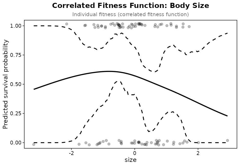

Figure 1. Correlated fitness function for body size

5.9 correlated_fitness_surface()

Purpose: Estimates 2D fitness surfaces using thin-plate splines (continuous) or GAMs (binary and count fitness).

correlated_fitness_surface(
  data,
  fitness_col,
  trait_cols, # Exactly 2 traits
  grid_n = 60, # Grid resolution (grid_n × grid_n points)
  method = "auto", # "auto", "gam", or "tps"
  scale_traits = FALSE, # Traits are normally standardised upstream
  group = NULL, # Optional grouping column, e.g. species or year
  group_effect = TRUE, # Group as a fixed effect in the model, or FALSE to use it only for the overlay
  k = NULL, # Basis dimension for the GAM smooth; set from the data if NULL
  mask = TRUE, # Leave grid points outside the data blank
  too_far = NULL, # Also blank cells farther than this share of the range from any individual
  bs = "tp", # GAM basis: "tp", "cr" or "ps"
  smoothing = "REML", # GAM smoothing parameter choice: "REML", "GCV.Cp" or "ML"
  clamp = TRUE, # Hold thin-plate predictions within the range of the fitness type
  level = 0.95, # Confidence level of the band around a GAM surface
  by_group = FALSE, # TRUE: a separate surface for each group, returned as a named list
  count_family = "poisson" # "quasipoisson" or "nb" for overdispersed counts
)

Method selection:

• "tps": Uses fields::Tps() for continuous fitness (spline-based)
• "gam": Uses mgcv::gam() with a thin-plate smooth and REML smoothing (works for all three). The family follows the fitness column: binomial for 0/1, Poisson with a log link for counts such as lifespan in years or offspring, Gaussian otherwise. Counts are often overdispersed. A Poisson fit warns when the dispersion is above 1.5, and count_family = "quasipoisson" then corrects the standard errors and peak comparisons. bs and smoothing swap in another basis or criterion to match a published analysis; with "cr" or "ps" the two traits enter as a tensor product.
• "auto": Chooses based on fitness type (GAM for binary and count, TPS for continuous)

Basis dimension: with k = NULL the GAM uses min(30, max(10, floor(sqrt(n1 * n2)))), where n1 and n2 are the numbers of distinct values of each trait, capped at one less than the number of observations. Pass an integer to override it.

Masking: the fitted surface is evaluated on a rectangular grid, and the corners of that rectangle are usually places no individual occupies. With mask = TRUE grid points outside the convex hull of the observed trait pairs get NA fitness, so the optimum is found within the data, and the plots draw the surface up to the hull and leave the outside blank. The grid keeps the unmasked predictions in .fit_all, records which points were kept in .inside, and the result carries the hull polygon in $hull. The hull still bridges gaps between separate clusters of individuals, such as two species on one surface. too_far adds the distance rule from mgcv::vis.gam: after scaling the grid to the unit square, cells farther than too_far from the nearest individual are blanked as well, and the distance is kept in .dist. Beausoleil et al. (2023) used 0.15. The default applies no distance rule.

Separate fits: by_group = TRUE, here and in univariate_spline(), fits each group on its own rows and returns a named list, rather than one shape shifted by a group term. Prepare the data with the same group so each is standardised on its own, and plot with lapply().

Groups: with group the GAM includes the column as a fixed effect and predicts the surface at the reference level, as the gradient models do for year or site. group_effect = FALSE fits one surface to everyone and uses the group only for the overlay, which is what a community surface of several species needs. The result’s $groups table gives, for each group, its size, its mean of both traits and the highest point of the surface within that group’s own convex hull, with peak_interior saying whether that point is a peak of the surface and peak_edge whether it sits at the edge of the data; when both are FALSE the surface keeps rising past the group’s range. The plots mark the means as labelled open circles and the peaks as triangles, filled for a peak and open otherwise, which is how Beausoleil et al. (2023) placed several species on one surface. $peaks lists every local maximum of the kept surface the same way, and the gold optimum becomes an open diamond when the highest cell sits at the edge of the data.

Returns: List containing:

• $model: Fitted model object
• $grid: Data frame with trait values, predicted fitness (.fit, masked), .fit_all and .inside; with the GAM also the standard error of the fit (.se) and its band (.fit_lo, .fit_hi)
• $hull: The convex hull of the data, used by the plots
• $original_data: The rows that were analysed
• $peaks: The local maxima of the kept surface, highest first, interior TRUE for a peak inside the data, FALSE for a maximum at its edge
• $groups: With group, one row per group with its mean traits and highest point, flagged peak_interior and peak_edge
• $method: Method used
• $k: Basis dimension used (GAM method)
• $data_type: “binary”, “count” or “continuous”

Example: survival is binary, so the raw 0/1 column goes in and a binomial GAM is fitted.

surface <- correlated_fitness_surface(
  data = prepared,
  fitness_col = "survival",
  trait_cols = c("size", "colour"),
  method = "gam"
)

# Find optimum (maximum fitness)
optimum <- surface$grid[which.max(surface$grid$.fit), ]
print(optimum)
#>            size    colour      .fit       .se  .fit_lo   .fit_hi  .fit_all
#> 2248 -0.3887548 0.5928513 0.7006815 0.1199263 0.432857 0.8777501 0.7006815
#>        .se_all .fit_lo_all .fit_hi_all .inside
#> 2248 0.1199263    0.432857   0.8777501    TRUE

5.10 plot_correlated_fitness()

Purpose: Visualise 2D fitness surfaces with contour plots.

plot_correlated_fitness(
  tps,                  # Output from correlated_fitness_surface()
  trait_cols,           # The two trait names
  bins = 12,            # Number of contour bins
  show_optimum = TRUE,  # Mark the highest fitness: gold diamond inside the data, open at its edge
  show_groups = TRUE,   # Mark group means and highest points when the surface has a group
  group_lines = TRUE,   # Dashed line from each group's mean to its peak
  uncertainty = "none", # "se": standard error lines; "band": lower, fit and upper panels
  ...                   # Passed to ggplot2::labs(), e.g. title or fill
)

plot_correlated_fitness_enhanced(
  tps,                  # Output from correlated_fitness_surface()
  trait_cols,
  original_data,        # Individuals to overlay, coloured by fitness
  fitness_col,
  bins = 12,
  uncertainty = "none"
)

Uncertainty: a GAM surface carries the standard error of its fitted fitness and a band around it, worked out on the scale of the link. uncertainty = "se" draws the standard error as dashed contour lines over the surface, and uncertainty = "band" draws the lower bound, the fit and the upper bound side by side on one fill scale. peak_difference(surface, from, to, valley = TRUE) gives the difference in fitted fitness between two points, given as group names or trait values, and between each of them and the pass between them, the lowest point on the highest route from one to the other, with standard errors from the covariance of the model’s coefficients. route = "line" takes the lowest point on the straight line instead, as Beausoleil et al. (2023) measured valley depths; ?peak_difference explains why the two can differ and why the comparisons are exploratory. The thin-plate spline gives no standard errors.

Example:

p <- plot_correlated_fitness(
  tps = surface,
  trait_cols = c("size", "colour"),
  bins = 12
)

print(p)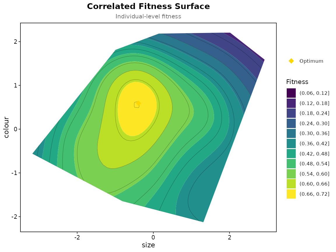

Correlated fitness surface for size and colour

p <- plot_correlated_fitness_enhanced(
  tps = surface,
  trait_cols = c("size", "colour"),
  original_data = prepared,
  fitness_col = "survival",
  bins = 12
)

print(p)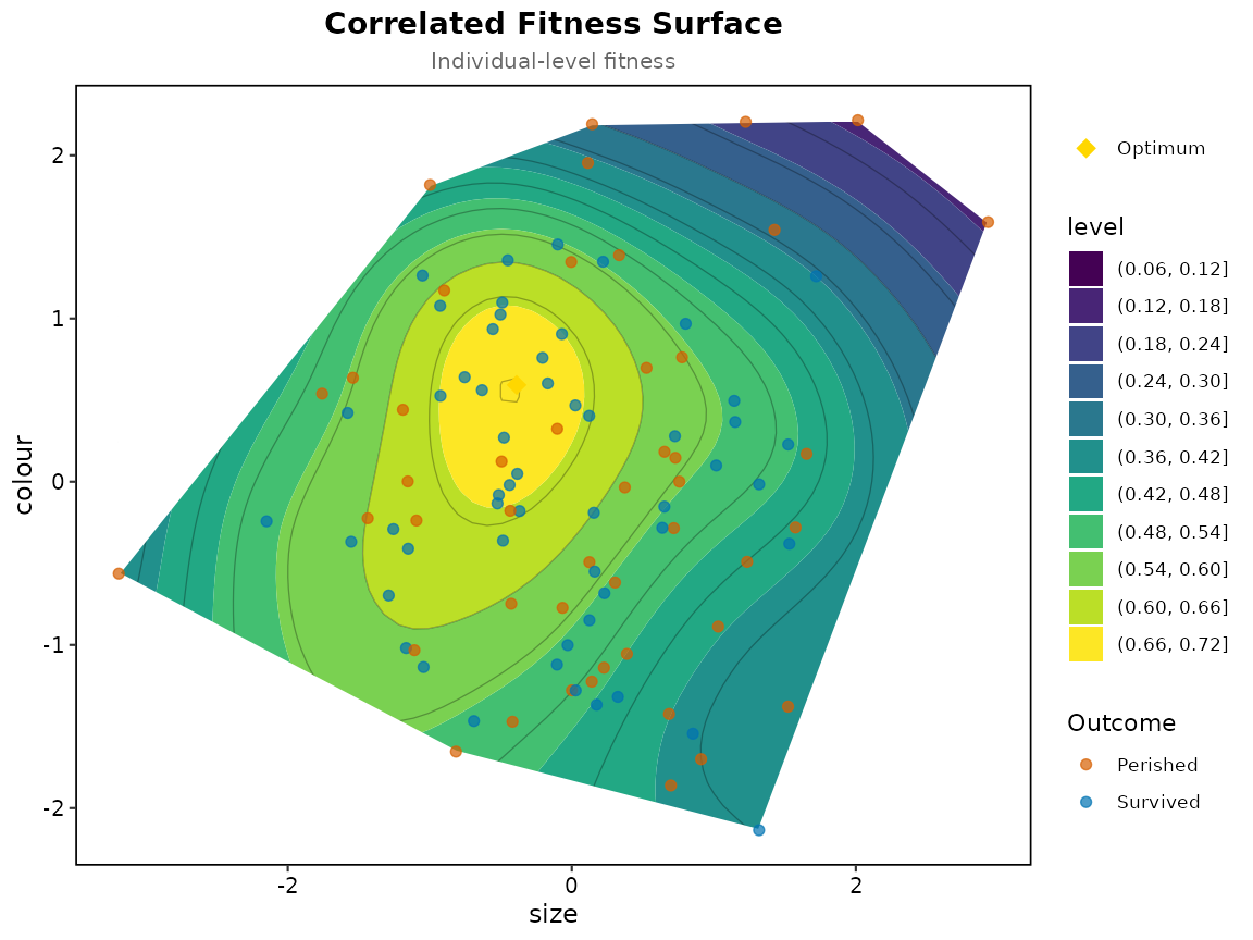

Correlated fitness surface with original data points

5.11 adaptive_landscape()

Purpose: Calculates the Wrightian adaptive landscape, which is a population-level concept distinct from correlated fitness surfaces.

adaptive_landscape(
  data,                      # Individual-level data frame
  fitness_model,             # $model from correlated_fitness_surface() or univariate_spline()
  trait_cols,                # One or two trait names
  group_col = NULL,          # Optional grouping column (e.g., "species")
  population_variance = NULL,# Within-population variance-covariance matrix
  simulation_n = 1000,       # Number of individuals to simulate per grid point
  grid_n = 50,               # Grid resolution (grid_n × grid_n)
  custom_range = NULL,       # Optional custom range for population means
  clamp = TRUE,              # Hold thin-plate fitness within the range of the fitness type
  support_warn = 0.25        # Share outside the data at the optimum that draws a note
)

Calculation Steps:

1. Create grid of possible population means ($\bar{z}_1$, $\bar{z}_2$) across the trait range
2. Estimate within-population variance from the data
3. Simulate individuals around each population mean: $\mathbf{z} \sim \mathrm{N}(\bar{\mathbf{z}}, \mathbf{P})$
4. Predict fitness for each simulated individual using the fitted model
5. Calculate mean fitness $\bar{W} = \frac{1}{N}\sum \hat{w}_{\text{ind}}$
6. Find the optimum, the population mean that maximises $\bar{W}$

The simulated populations spread beyond the data, more so towards the edge of the grid, and the fitness of those individuals is extrapolated. The function reports how far this goes, as the share of each simulated population falling outside the convex hull of the observed traits, and says so when the optimum rests on it.

Returns:

• $grid: Population means with mean fitness (.mean_fit); with one trait also the fitness function at those means (.ind_fit)
• $optimum: Population mean with highest fitness
• $support: Share of simulated individuals outside the data, over the grid (outside) and at the optimum (at_optimum); per population mean in the grid’s .outside
• $actual_population_means: Actual means (if group_col provided)

An optimum on the edge of the grid: this usually means the true optimum lies outside the observed traits. custom_range, a named list with one range per trait, moves or widens the grid, but fitness out there is extrapolated, and $support says how much of the simulated population that involves.

With a single trait the grid is a line of population means, the model is normally the $model of univariate_spline(), and the result is a curve rather than a surface.

Example:

landscape <- adaptive_landscape(
  data = prepared,
  fitness_model = surface$model,
  trait_cols = c("size", "colour"),
  grid_n = 50,
  simulation_n = 1000
)

landscape$optimum
#>           size      colour .mean_fit .outside
#> 1222 -0.741549 -0.02229907 0.5612512    0.143

5.12 plot_adaptive_landscape()

Purpose: Creates a 2D contour map showing how mean fitness varies with population mean phenotypes, or, for a single trait, a curve of mean fitness against the population mean with the fitness function drawn dashed alongside it.

plot_adaptive_landscape(
  landscape,                  # Output from adaptive_landscape()
  trait_cols,                 # One or two trait column names
  original_data = NULL,       # Optional original data for overlaying points
  group_col = NULL,           # Optional grouping column for labels
  bins = 12,                  # Number of contour bins
  show_optimum = TRUE,        # Show optimal population mean (gold diamond)
  show_actual_means = TRUE,   # Show actual population means (red points)
  show_individual = TRUE,     # One trait: also draw the fitness function
  show_support = FALSE,       # Mark where most of the simulated population leaves the data
  support_level = 0.5         # The share outside the data at which that line is drawn
)

plot_adaptive_landscape_3d(
  landscape,                  # Output from adaptive_landscape()
  trait_cols,                 # Two trait column names
  theta = -30,                # Azimuthal rotation angle
  phi = 30                    # Colatitude tilt angle
)

Example:

p <- plot_adaptive_landscape(
  landscape = landscape,
  trait_cols = c("size", "colour"),
  bins = 12
)

print(p)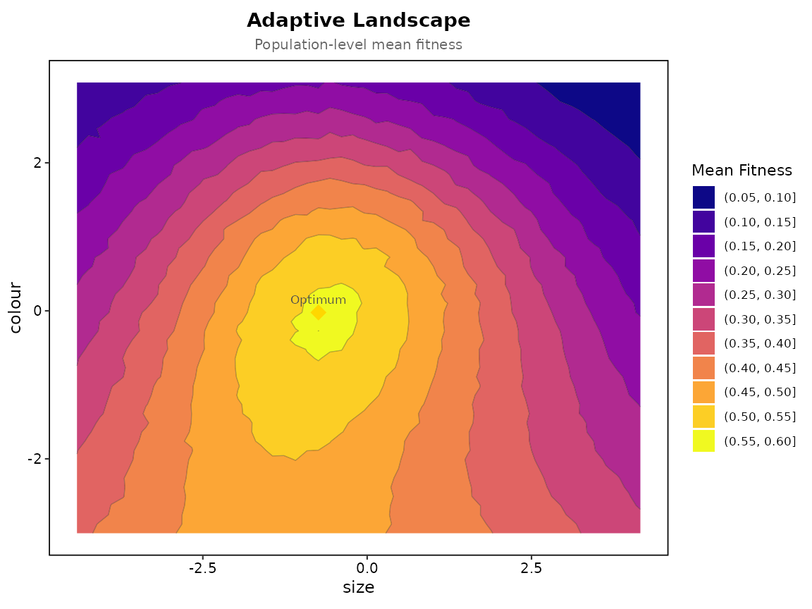

Adaptive landscape showing mean fitness as function of population mean size and colour

plot_adaptive_landscape_3d(
  landscape = landscape,
  trait_cols = c("size", "colour"),
  theta = -30,
  phi = 30
)

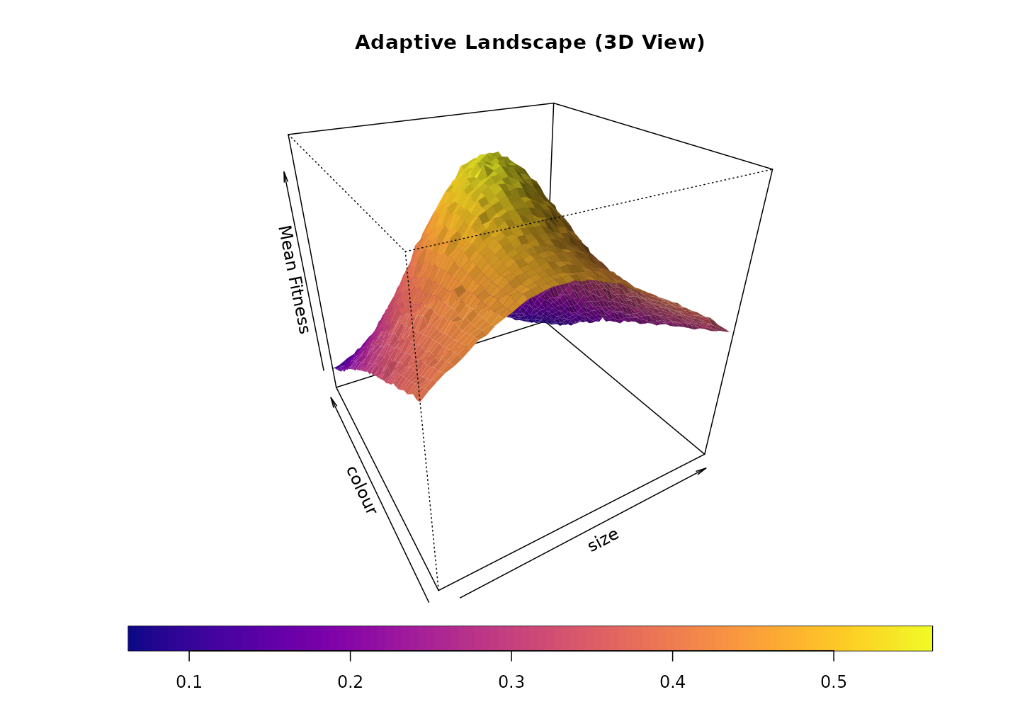
3D adaptive landscape showing the shape of mean fitness

5.13 selection_coefficients()

Purpose: Main wrapper function that runs a complete selection analysis.

selection_coefficients(
  data,
  fitness_col,
  trait_cols,
  fitness_type = c("auto", "binary", "count", "continuous"),
  standardize = TRUE,
  group = NULL,               # optional grouping column (e.g. year)
  use_relative_for_fit = TRUE,
  return_grouped = FALSE,     # TRUE: one set of gradients per group
  se_type = "ols"             # "hc3": leave-one-out standard errors
)

Workflow:

1. Prepares data (standardisation, relative fitness)
2. Detects fitness type (if auto)
3. Runs linear selection analysis
4. Runs nonlinear selection analysis
5. Extracts all coefficients into a single table

Returns: Data frame with columns:

• Term: Coefficient name (e.g., “size”, “size²”, “size×colour”)
• Type: “Linear”, “Quadratic”, or “Correlational”
• Beta_Coefficient: Estimated selection gradient
• Standard_Error: Standard error of estimate, least squares or HC3 (se_type)
• P_Value: Statistical significance
• Variance: Square of standard error

se_type = "hc3" gives leave-one-out standard errors (MacKinnon & White, 1985; Mitchell-Olds & Shaw, 1987; see ?selection_coefficients). They allow for residual spread that changes with the traits, as it does when the model leaves out curvature; in the package’s simulation they recovered most of the coverage lost there, most of all with heavy-tailed traits. They did nothing for the coverage lost to estimating a skewed trait’s SD, and with survival and counts they covered a little less. For continuous fitness the p-values follow them; for survival and counts the p-values come from the GLM with either se_type.

Example:

results_binary <- selection_coefficients(
  data = prepared,
  fitness_col = "survival", # Binary 0/1
  trait_cols = c("size", "colour"), # Only available traits
  fitness_type = "binary",
  standardize = TRUE
)

print(results_binary)
#>            Term          Type Beta_Coefficient Standard_Error    P_Value
#> 1          size        Linear    -0.1137115929     0.09366118 0.22486021
#> 2        colour        Linear    -0.0006673983     0.09366118 0.99313501
#> 3         size²     Quadratic    -0.1923255937     0.13409909 0.14687155
#> 4       colour²     Quadratic    -0.3230714003     0.16086280 0.04719178
#> 5 size × colour Correlational     0.0051607761     0.10537314 0.91801711
#>      Variance
#> 1 0.008772416
#> 2 0.008772416
#> 3 0.017982567
#> 4 0.025876841
#> 5 0.011103499

The table is put together by three exported helpers, extract_linear_coefficients(), extract_quadratic_coefficients() and extract_interaction_coefficients(). Each takes the trait names and the model object from analyze_linear_selection() or analyze_nonlinear_selection(), pulls the terms out by name, doubles the quadratic estimates and skips any term the model does not have. They are only needed if you fit the models yourself and want the same table.

5.14 selection_report()

selection_coefficients() gives the coefficient table and selection_report() the differentials and gradients in one standardised table:

selection_report(prepared, "survival", c("size", "colour"), fitness_type = "binary")
#> Selection analysis (standardised traits, relative fitness)
#> Fitness type: binary 
#> p-values are from a logistic model on the same terms
#> 
#>           Term          Type Estimate Std_Error P_Value Sig
#>           size  Differential  -0.1126        NA      NA    
#>         colour  Differential  -0.0078        NA      NA    
#>           size        Linear  -0.1137    0.0937  0.2249    
#>         colour        Linear  -0.0007    0.0937  0.9931    
#>          size²     Quadratic  -0.1923    0.1341  0.1469    
#>        colour²     Quadratic  -0.3231    0.1609  0.0472   *
#>  size × colour Correlational   0.0052    0.1054  0.9180    
#> 
#> Signif: *** 0.001  ** 0.01  * 0.05  . 0.1

5.15 compare_fitness_surfaces_data()

Purpose: Compares the individual-level fitness surface with the population-level adaptive landscape: their optima, the distance between them, summary statistics and the correlation between the two surfaces. The surface is selection on individuals and the landscape is where the population mean would move, so the two can peak in different places.

comparison <- compare_fitness_surfaces_data(
  correlated_surface = surface,
  adaptive_landscape = landscape,
  trait_cols = c("size", "colour")
)

comparison$summary_stats
#>              Surface Fitness_Range_Min Fitness_Range_Max Fitness_Mean
#> 1 Correlated Fitness        0.17063668         0.7006815    0.4908177
#> 2 Adaptive Landscape        0.06221752         0.5612512    0.3493286
#>   Fitness_SD N_Points
#> 1  0.1185462     3600
#> 2  0.1226478     2500

plots <- plot_fitness_surfaces_comparison(
  comparison_data = comparison,
  bins = 15
)

print(plots$overlay)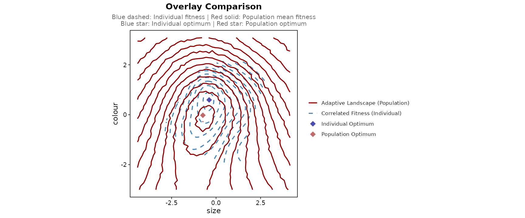

Overlay comparison

plots <- plot_fitness_surfaces_comparison(
  comparison_data = comparison,
  bins = 15
)

print(plots$side_by_side)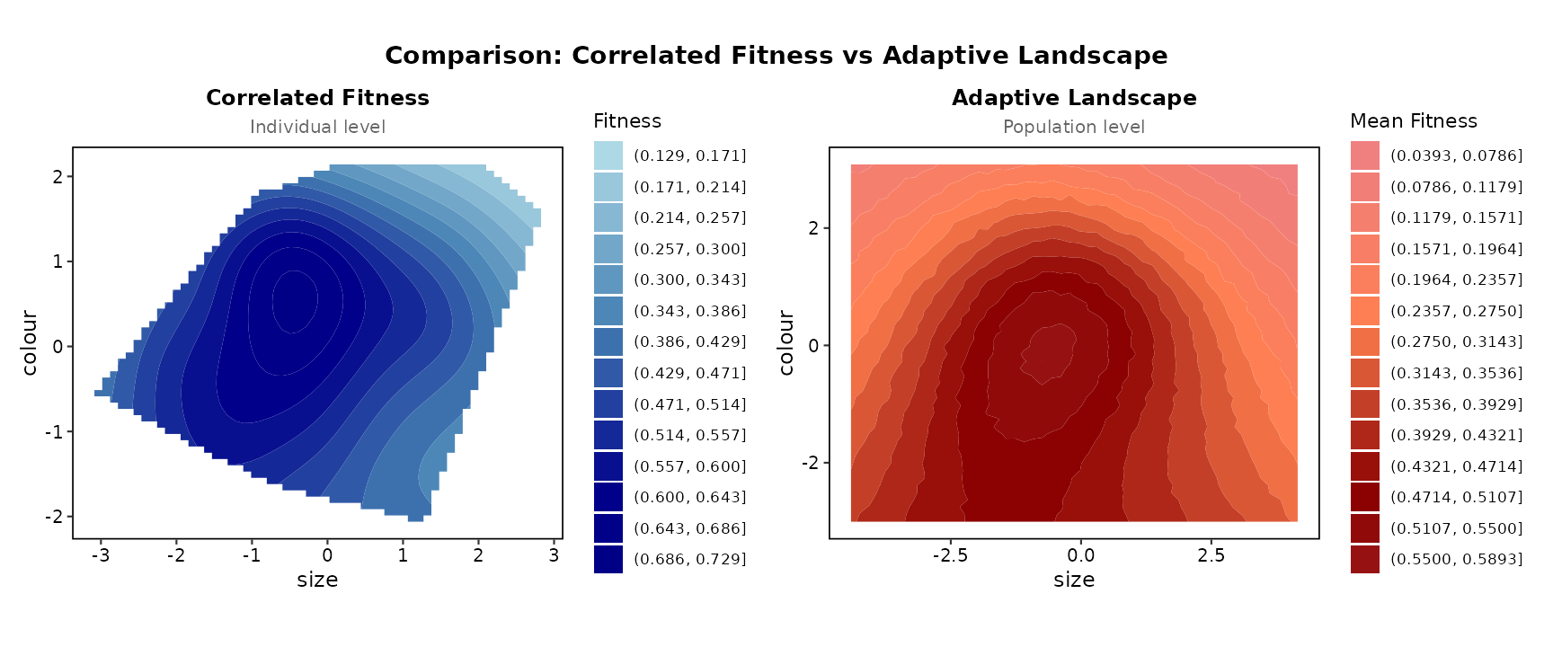

Side-by-side comparison

---

5.16 temporal_landscape() and plot_temporal_landscape()

Purpose: Fit the fitness function or surface, and optionally the adaptive landscape, separately for each period, to see how selection changes over time.

temporal_landscape(
  data,                  # Traits standardised once, over all periods
  fitness_col,
  trait_cols,            # One or two traits
  time_col,              # The period of each row, usually year
  fitness_type = "auto",
  min_n = 20,            # Periods with fewer rows are skipped
  landscape = TRUE,      # Also the adaptive landscape per period
  bootstrap = FALSE,     # Band around each period's fitness function (one trait)
  grid_n = 60, simulation_n = 300
)

plot_temporal_landscape(
  tl,
  type = "panels",       # or "heatmap" for one trait
  show_points = TRUE, show_landscape = TRUE, show_optimum = TRUE,
  ncol = NULL            # Panel columns
)

Returns: a list with one fit and one landscape per period, a summary table (n, mean fitness, trait means, the smooth’s degrees of freedom, the position and height of the highest fitness and whether it sits at the edge of the data, the number of interior peaks for one trait, and the landscape optimum), the fitted values of every period stacked in grid, for one trait the fitness functions on a common grid in heat (blank where a period has no individuals), and the periods skipped for having fewer than min_n rows.

Standardise the traits once over all periods before calling; nothing is restandardised per period, since the periods share one trait axis. The number of peaks depends on the basis size k and the smoothing criterion, as any spline feature does, so test disruptive selection with the quadratic gradient on the birds between the peaks, as Beausoleil et al. (2019) did.

Example: medium ground finches at El Garrapatero, one row per bird per year it was seen, survival (seen again in any later year) against beak size (first principal component of the three beak medians), from the public data of Beausoleil et al. (2019). The splines here use REML; the “Finches year by year” article compares it with UBRE.

finch_prep <- prepare_selection_data(finch_yearly, "survived", "beak_pc1")
years <- temporal_landscape(finch_prep, "survived", "beak_pc1", "year", smoothing = "REML", simulation_n = 200)

years$summary[, c("time", "n", "mean_fitness", "edf", "optimum_beak_pc1", "peaks")]
#>   time   n mean_fitness      edf optimum_beak_pc1 peaks
#> 1 2004 110    0.3454545 1.000082        -1.834495     0
#> 2 2005 185    0.2756757 1.000645        -1.708023     0
#> 3 2006 233    0.1802575 1.000176        -2.045747     0
#> 4 2007  61    0.3442623 1.016109        -1.162755     0
#> 5 2008 127    0.3070866 1.000084        -2.103969     0
#> 6 2009 196    0.1938776 3.165374         2.841979     1
#> 7 2010 175    0.1885714 1.000047        -2.103969     0

plot_temporal_landscape(years, ncol = 4)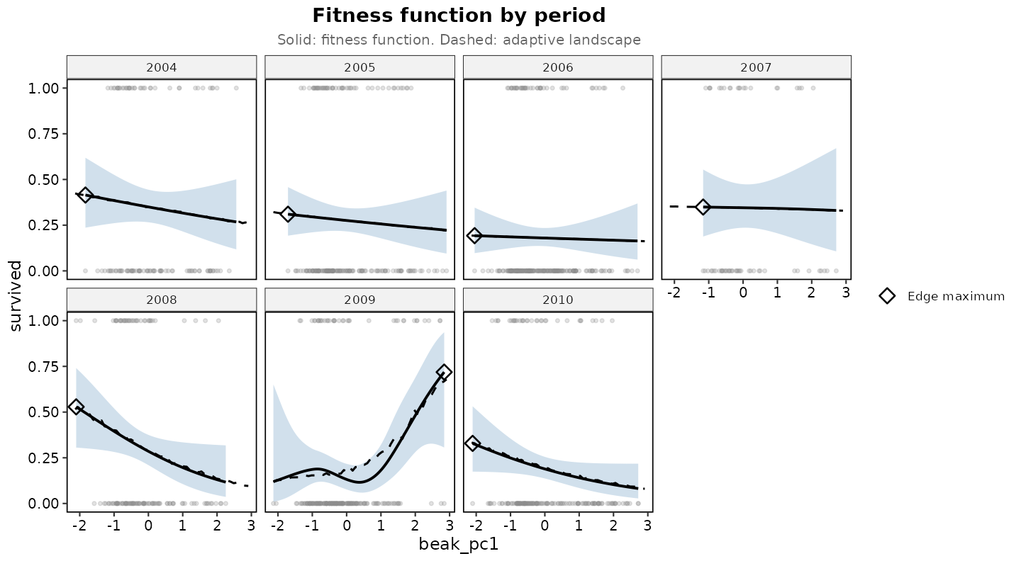

Survival against beak size, one panel per year. Solid: fitness function. Dashed: adaptive landscape. Diamond: highest survival.

plot_temporal_landscape(years, type = "heatmap")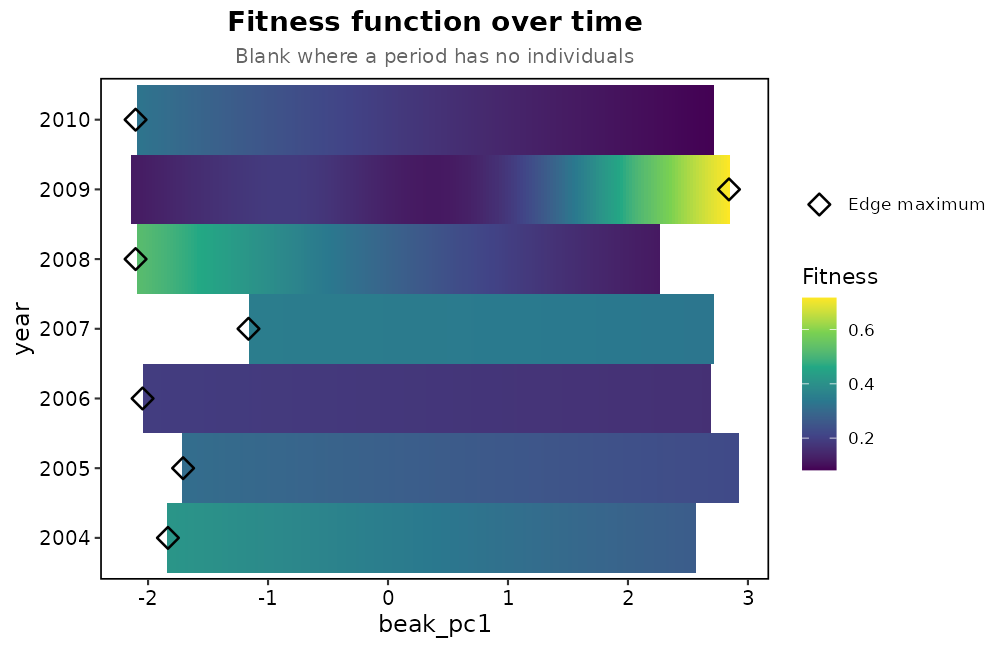

The same fitness functions as a heat map, blank where a year has no birds.

With REML the functions are close to straight lines on the logit scale in every year but 2009, when survival dips past a small bump for the small morph and then rises steeply towards large beaks; Beausoleil et al. (2019) found their deepest valley in the 2009 to 2010 interval. With the default UBRE criterion 2005, 2006 and 2008 each show two or three peaks instead. Their test was the quadratic gradient on the birds between the peaks, which is analyze_disruptive_selection() in section 5.6 run on that subset.

5.17 canonical_analysis() and plot_canonical_axes()

Purpose: Rotate the matrix of quadratic and correlational gradients to its canonical axes and read the curvature along each.

canonical_analysis(
  data, fitness_col, trait_cols,
  fitness_type = "auto",
  standardize = TRUE,
  group = NULL,        # Standardise and relativise within groups, as the gradients do
  bootstrap = FALSE,   # Percentile intervals for the eigenvalues
  n_boot = 200,
  conf = 0.95,
  test = "permutation", # p-values by shuffling fitness (Reynolds et al. 2010); "double_regression" for the double-regression tests
  n_perm = 999
)

Returns: the gamma matrix, $\beta$, the loadings M with one column per axis, and an axes table with each eigenvalue $\lambda$, its standard error from the double regression of Bisgaard and Ankenman (1996), a p-value from the permutation test of Reynolds et al. (2010), and the directional selection along the axis, $\theta = \mathbf{M}^\top\boldsymbol{\beta}$. The prepared data come back with the canonical scores m1, m2, … added.

set.seed(1)
ca <- canonical_analysis(bumpus, "survival", c("total_length", "weight", "humerus"))
ca
#> Canonical analysis of gamma for total_length, weight, humerus on 136 individuals
#> 
#> Loadings (columns are the canonical axes):
#>                  m1     m2    m3
#> total_length -0.256 -0.056 0.965
#> weight        0.590  0.782 0.202
#> humerus       0.766 -0.621 0.167
#> 
#> Curvature along each axis (negative is consistent with stabilising selection, positive with disruptive):
#>  axis  lambda     se p_value  theta
#>    m1  0.0331 0.1138   0.968  0.281
#>    m2 -0.0248 0.2509   0.905 -0.507
#>    m3 -0.1511 0.0988   0.469 -0.282
#> 
#> p-values from 999 permutations of fitness (Reynolds et al. 2010), which allow for the 
#> axes coming from these data. The standard errors treat the axes as known.

A negative $\lambda$ is curvature along that axis, consistent with stabilising selection, and a positive one with disruptive selection, exactly as for $\gamma_{ii}$. The double-regression tests treat the axes as known when they were estimated from the same data, which makes them much too liberal (Reynolds et al., 2010). The p-values come from shuffling fitness among individuals and repeating the analysis each time; set a seed first to get the same p-values again. Sampling error in $\boldsymbol{\gamma}$ also spreads its eigenvalues, so the largest curvatures are overestimated, more so with many traits and few individuals (Reynolds et al., 2010), and the estimated axes lean towards directions of phenotype with little variance (Morrissey, 2014). bootstrap = TRUE gives percentile intervals, with each resample’s axes matched to the original ones, and plot_canonical_axes() draws the fitness surface along any two axes, or the fitness function along one, which is where to check whether a curved axis has a peak inside the data.

plot_canonical_axes(ca, which = c(1, 3), grid_n = 30)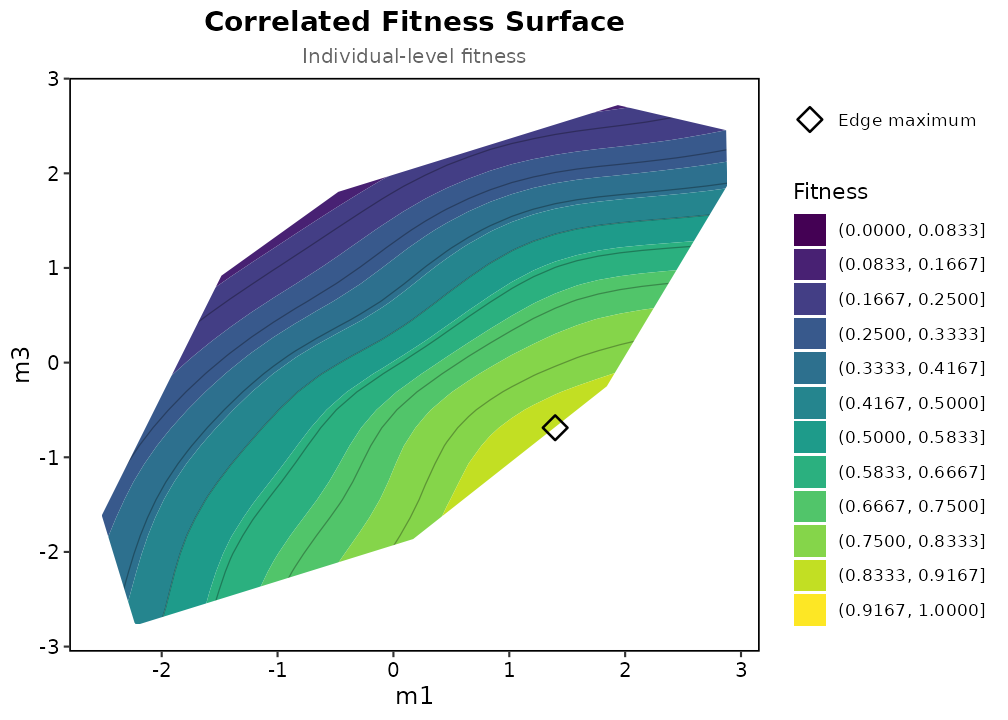

Fitness surface along the first and last canonical axes

---

6. Interpretation Guide

6.1 Statistical Significance

The p-values test whether each gradient differs from zero. Treat them as a guide to how much the data say, not as the size of selection: a gradient of 0.05 with p < 0.001 is well estimated but weak, and a gradient of 0.4 with p = 0.08 may matter more. Report the estimate and its standard error or bootstrap interval alongside the p-value.

6.2 Selection Types

Linear Selection ($\beta$):

$\beta$ sign	Interpretation
Positive (+)	Selection favours larger trait values
Negative (-)	Selection favours smaller trait values
Zero (0)	No directional selection

Quadratic Selection ($\gamma$):

$\gamma$ sign	Interpretation	Shape
Negative (-)	Stabilising selection	∩-shaped
Positive (+)	Disruptive selection	∪-shaped
Zero (0)	No nonlinear selection	Linear

Correlational Selection ($\gamma_{ij}$):

$\gamma_{ij}$ sign	Interpretation	Shape of the surface
Positive (+)	Selection favours positive correlation (both traits high or both low)	A ridge running from low-low to high-high; the two off-diagonal corners are valleys
Negative (-)	Selection favours negative correlation (one high, one low)	A ridge running from high-low to low-high
Zero (0)	No correlational selection on the pair	Contours are symmetric about both axes

In Brodie’s (1992) garter snakes, neither colour pattern nor escape behaviour was under strong selection on its own, but striped snakes that fled in a straight line and unstriped snakes that reversed direction both survived better than the mismatched combinations. Selection was on the combination, which shows as a ridge across the fitness surface with no peak on either axis. The sign of $\gamma_{ij}$ depends on how the traits are scored. With stripes scored high and reversals counted, the favoured pairs are high-low and low-high, so the gradient is negative.

6.3 Effect Sizes

For standardised traits ($\mu=0, \sigma=1$):

$|\beta|$	Effect size
< 0.1	Weak selection
0.1 - 0.3	Moderate selection
> 0.3	Strong selection

These bands are relative to the published record: across the studies collated by Kingsolver et al. (2001) the median $|\beta|$ was 0.16 and the median $|\gamma|$ was 0.10, so a gradient above 0.3 is stronger than most selection measured in the wild. Gradients standardised by the trait mean instead of its standard deviation put traits with different variances on one scale, and Hereford et al. (2004) collate the record on that scale; the package reports variance-standardised gradients only.

6.4 Example Interpretations

Scenario 1: β_size = 0.25, p = 0.001
→ "Body size experiences significant positive directional selection.
   A one-standard-deviation increase in size increases relative fitness by 0.25 units."

Scenario 2: γ_size = -0.15, p = 0.02
→ "Fitness curves downwards with body size, which is consistent with
   stabilising selection if the fitness function peaks inside the data."

Scenario 3: γ_size x beak = 0.32, p = 0.004
→ "Significant positive correlational selection between size and beak depth.
   Selection favours individuals that are either both large or both small."

---

7. Troubleshooting and Common Issues

7.0 Assumption Checks

check_selection_assumptions() puts the checks behind a Lande and Arnold analysis in one table: Mardia’s tests of multivariate normality of the traits, which is what lets the gradients be read as the slope and curvature of the fitness surface (Lande & Arnold, 1983; Morrissey & Sakrejda, 2013; they equal $\mathbf{P}^{-1}\mathbf{S}$ by least squares whatever the distribution), Shapiro-Wilk for each trait, the largest VIF, the individuals (for survival, the rarer outcome) per quadratic term, and for the gradient models residual normality and heteroscedasticity, separation, or the dispersion ratio. With the performance package installed it adds that package’s heteroscedasticity and overdispersion tests and an R squared. Report the table with the gradients, as Palacio et al. (2019) ask.

check_selection_assumptions(bumpus, "survival", c("total_length", "weight", "humerus"))
#> Assumption checks (binary fitness, n = 136)
#> 
#>  check                                    statistic p    
#>  Multivariate normality: Mardia skewness  1.05      0.006
#>  Multivariate normality: Mardia kurtosis    15      0.997
#>  Normality of total_length (Shapiro-Wilk) 0.978     0.029
#>  Normality of weight (Shapiro-Wilk)       0.97      0.004
#>  Normality of humerus (Shapiro-Wilk)      0.98      0.048
#>  Collinearity: largest VIF                1.75           
#>  Rarer outcome per quadratic term         7.11           
#>  Logistic model: separation               1.34           
#>  Model fit: R2_Tjur (performance)         0.24           
#>  note                                                      
#>  skewed                                                    
#>  no evidence against normality                             
#>  not normal                                                
#>  not normal                                                
#>  not normal                                                
#>  below 5                                                   
#>  64 of the rarer outcome for 9 terms; treat gamma with care
#>  no sign of separation                                     
#> 

7.1 Sample Size Recommendations

Analysis	Minimum n	Recommended n
Linear selection (continuous)	10	> 30
Linear selection (binary)	20 per group	> 50 per group
Nonlinear selection	20	> 100
Bivariate TPS	30	> 200

The nonlinear model grows quickly with the number of traits: $m$ traits give $m$ linear, $m$ quadratic and $m(m-1)/2$ correlational terms, so nine traits mean 54 terms. Allow about ten individuals per term, and for binary fitness about ten survivors (or deaths, whichever is rarer) per term; below that the quadratic and correlational estimates are mostly noise, even when their p-values are small. Choose fewer traits on biological grounds rather than fitting them all.

7.2 Convergence Issues in Binary Models

Symptoms:

• Very large coefficients (> 10)
• Extremely large standard errors
• Warning about “complete separation”

Solutions:

# 1. Check for complete separation
table(data$fitness, cut(data$trait, 5))

# 2. Use Firth's penalised likelihood
if (!require("logistf")) install.packages("logistf")
library(logistf)
fit <- logistf(fitness ~ trait, data = data)

# 3. Collect more data
# 4. Simplify model (fewer traits)

7.3 Missing Data

prepare_selection_data() checks the fitness and trait columns for NA. The default, na_action = "warn", keeps every row and warns with the count. The models drop incomplete rows themselves, and traits and relative fitness are standardised on the rows that are analysed, so the rows that fall out do not shift the means. Rows with a missing group label are kept and treated as their own group. na_action = "drop" removes incomplete rows up front and prints how many went, which keeps the sample size explicit and is the better choice when the same data go on to the splines and surfaces.

# Missing values per column, and incomplete rows
colSums(is.na(data[, c(fitness_col, trait_cols)]))
sum(!complete.cases(data[, c(fitness_col, trait_cols)]))

prepared <- prepare_selection_data(data, fitness_col, trait_cols, na_action = "drop")

Imputing traits is possible but changes what is being estimated. With more than a few percent of rows incomplete, report the count and analyse the complete cases.

7.4 Multicollinearity

High correlations between traits can inflate standard errors:

# Check correlations
cor(data[, trait_cols])

# Calculate VIF
if (requireNamespace("car", quietly = TRUE)) {
  vif_vals <- car::vif(model)
  # VIF > 5 is flagged by the package; > 10 is serious
}

Solutions:

• Use ridge regression
• Collect more data

7.5 Reduced k Warning

univariate_spline() warns “Reducing k from 10 to …” when a trait has fewer distinct values than the basis asks for, which happens with small groups, single years or coarsely measured traits. The curve is then less flexible than the default. To set the basis size yourself, in the spline or the surface:

uni <- univariate_spline(prepared, "survival", "size", k = 5)
surface <- correlated_fitness_surface(prepared, "survival", c("size", "colour"), k = 15)

---

8. References

1. Lande, R., & Arnold, S. J. (1983). The measurement of selection on correlated characters. Evolution, 37(6), 1210-1226.

2. Stinchcombe, J. R., Agrawal, A. F., Hohenlohe, P. A., Arnold, S. J., & Blows, M. W. (2008). Estimating nonlinear selection gradients using quadratic regression coefficients: double or nothing? Evolution, 62(9), 2435-2440.

3. Schluter, D. (1988). Estimating the form of natural selection on a quantitative trait. Evolution, 42(5), 849-861.

4. Brodie, E. D. (1992). Correlational selection for color pattern and antipredator behavior in the garter snake Thamnophis ordinoides. Evolution, 46(5), 1284-1298.

5. Kingsolver, J. G., Hoekstra, H. E., Hoekstra, J. M., Berrigan, D., Vignieri, S. N., Hill, C. E., Hoang, A., Gibert, P., & Beerli, P. (2001). The strength of phenotypic selection in natural populations. The American Naturalist, 157(3), 245-261.

6. Wood, S. N. (2017). Generalized Additive Models: An Introduction with R (2nd ed.). Chapman and Hall/CRC.

7. Brodie, E. D., III, & Janzen, F. J. (1996). On the assignment of fitness values in statistical analyses of selection. Evolution, 50(1), 437-442.

8. Brodie, E. D., III, Moore, A. J., & Janzen, F. J. (1995). Visualizing and quantifying natural selection. Trends in Ecology & Evolution, 10(8), 313-318.

9. Schluter, D., & Nychka, D. (1994). Exploring fitness surfaces. The American Naturalist, 143(4), 597-616.

10. Palacio, F. X., Ordano, M., & Benitez-Vieyra, S. (2019). Measuring natural selection on multivariate phenotypic traits: a protocol for verifiable and reproducible analyses of natural selection. Israel Journal of Ecology & Evolution, 65, 130-136. doi:10.1163/22244662-20191064

11. Svensson, E. I. (2023). Phenotypic selection in natural populations: what have we learned in 40 years? Evolution, 77(7), 1493-1504.

12. Mardia, K. V. (1970). Measures of multivariate skewness and kurtosis with applications. Biometrika, 57(3), 519-530.

13. Beausoleil, M.-O., Carrión, P. L., Podos, J., Camacho, C., Rabadán-González, J., Richard, R., Lalla, K., Raeymaekers, J. A. M., Knutie, S. A., De León, L. F., Chaves, J. A., Clayton, D. H., Koop, J. A. H., Sharpe, D. M. T., Gotanda, K. M., Huber, S. K., Barrett, R. D. H., & Hendry, A. P. (2023). The fitness landscape of a community of Darwin’s finches. Evolution, 77(12), 2533-2546.

14. Beausoleil, M.-O., Frishkoff, L. O., M’Gonigle, L. K., Raeymaekers, J. A. M., Knutie, S. A., De León, L. F., Huber, S. K., Chaves, J. A., Clayton, D. H., Koop, J. A. H., Podos, J., Sharpe, D. M. T., Hendry, A. P., & Barrett, R. D. H. (2019). Temporally varying disruptive selection in the medium ground finch (Geospiza fortis). Proceedings of the Royal Society B, 286(1916), 20192290.

15. Arnold, S. J., & Wade, M. J. (1984). On the measurement of natural and sexual selection: theory. Evolution, 38(4), 709-719.

16. Hereford, J., Hansen, T. F., & Houle, D. (2004). Comparing strengths of directional selection: how strong is strong? Evolution, 58(10), 2133-2143.

17. Morrissey, M. B., & Sakrejda, K. (2013). Unification of regression-based methods for the analysis of natural selection. Evolution, 67(7), 2094-2100.

18. Phillips, P. C., & Arnold, S. J. (1989). Visualizing multivariate selection. Evolution, 43(6), 1209-1222.

19. Blows, M. W., & Brooks, R. (2003). Measuring nonlinear selection. The American Naturalist, 162(6), 815-820.

20. Bisgaard, S., & Ankenman, B. (1996). Standard errors for the eigenvalues in second-order response surface models. Technometrics, 38(3), 238-246.

21. Reynolds, R. J., Childers, D. K., & Pajewski, N. M. (2010). The distribution and hypothesis testing of eigenvalues from the canonical analysis of the gamma matrix of quadratic and correlational selection gradients. Evolution, 64(4), 1076-1085.

22. Morrissey, M. B. (2014). In search of the best methods for multivariate selection analysis. Methods in Ecology and Evolution, 5(10), 1095-1109.

23. Bumpus, H. C. (1899). The elimination of the unfit as illustrated by the introduced sparrow, Passer domesticus. Biological Lectures, Marine Biological Laboratory, Woods Hole, 209-226.

24. Martin, C. H. (2016). Context dependence in complex adaptive landscapes: frequency and trait-dependent selection surfaces within an adaptive radiation of Caribbean pupfishes. Evolution, 70(6), 1265-1282.

25. MacKinnon, J. G., & White, H. (1985). Some heteroskedasticity-consistent covariance matrix estimators with improved finite sample properties. Journal of Econometrics, 29(3), 305-325.

26. Mitchell-Olds, T., & Shaw, R. G. (1987). Regression analysis of natural selection: statistical inference and biological interpretation. Evolution, 41(6), 1149-1161.