Plot fitness functions and landscapes over time

Usage

plot_temporal_landscape(
  tl,
  type = c("panels", "heatmap"),
  show_points = TRUE,
  show_landscape = TRUE,
  show_optimum = TRUE,
  connect = FALSE,
  bins = 10,
  ncol = NULL,
  ...
)

Arguments

tl: Output of temporal_landscape().
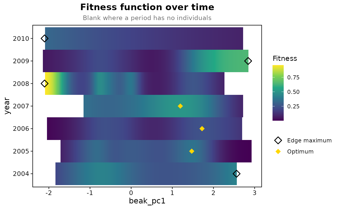
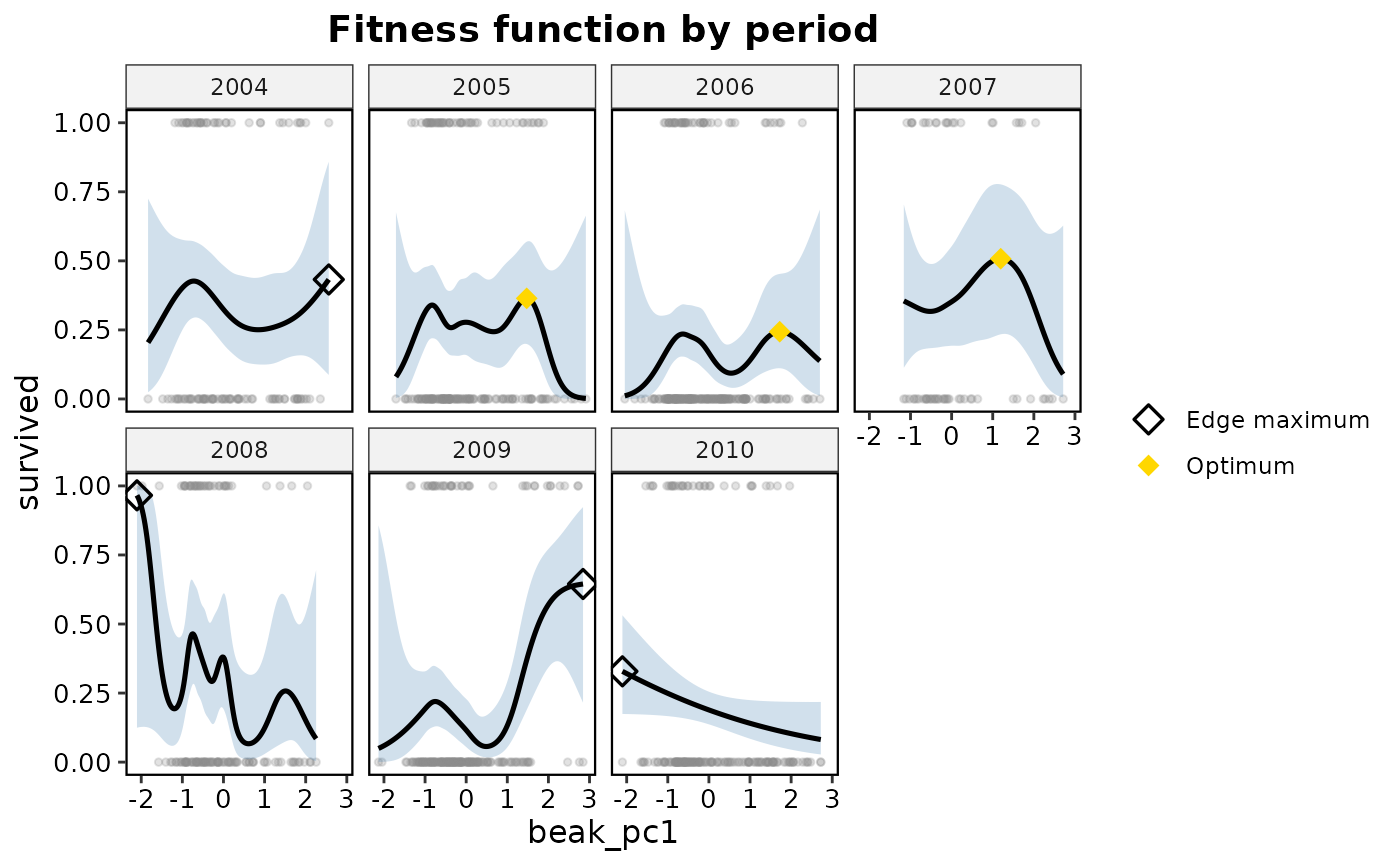
type: "panels" draws one panel per period: the fitness function with its band and the individuals for one trait, the fitness surface for two. "heatmap", for one trait only, draws fitness against trait and period in one panel, with the position of the highest fitness in each period marked.
show_points: Logical; draw the individuals in each panel.
show_landscape: Logical; for one trait, also draw each period's adaptive landscape as a dashed curve.
show_optimum: Logical; mark the highest fitted fitness in each period, as a gold diamond when it lies inside the data and an open one when it sits at the edge of the range.
connect: Logical; in the heat map, join the highest fitness of successive periods with a line. Default is FALSE, since a maximum at the edge of the range is not a peak.
bins: Contour bins for two-trait panels.
ncol: Number of panel columns.
...: Additional arguments passed to ggplot2::labs().

Value

A ggplot object.

Examples

prep <- prepare_selection_data(finch_yearly, "survived", "beak_pc1")
years <- temporal_landscape(prep, "survived", "beak_pc1", "year", landscape = FALSE)
#> 2004: n = 110, mean fitness 0.345, edf 3.0, 1 interior peak, highest fitness at the edge of the data
#> 2005: n = 185, mean fitness 0.276, edf 5.2, 3 interior peaks
#> 2006: n = 233, mean fitness 0.180, edf 4.4, 2 interior peaks
#> 2007: n = 61, mean fitness 0.344, edf 2.7, 1 interior peak
#> 2008: n = 127, mean fitness 0.307, edf 7.0, 3 interior peaks, highest fitness at the edge of the data
#> 2009: n = 196, mean fitness 0.194, edf 4.8, 1 interior peak, highest fitness at the edge of the data
#> 2010: n = 175, mean fitness 0.189, edf 1.0, 0 interior peaks, highest fitness at the edge of the data
plot_temporal_landscape(years, ncol = 4)

plot_temporal_landscape(years, type = "heatmap")