
Beausoleil et al. (2023) fitted one fitness surface to 3428 ground
finches at El Garrapatero on Santa Cruz: four species, with Geospiza
fortis split into its small and large beak morphs, five groups in
all. Fitness was apparent lifespan, the last year a bird was seen minus
the first, and the traits were beak length and depth in millimetres.
finch_community holds the data, with the year each bird was
first caught, built from their archive (doi:10.5683/SP3/0YIWSE). The 172 birds first caught in
2020, the last year of the archive, could not be seen again and have a
lifespan of 0; they are among the 3428, so they stay in, except in the
comparison with capture year below.
##
## fortis large fortis small   fuliginosa magnirostris     scandens
##          586         1384         1096           53          309
One pooled surface, the groups marked
The traits stay in millimetres (the first two warnings below note this), the fitness type is detected as a count so the surface takes a Poisson family as in their model, cells farther than 0.15 of the axis range from any bird are blanked as in their code, and the group is used only to mark each group’s mean and the highest point of the surface within its own range. A pooled surface like this can’t tell the beak apart from other differences between the species.
surface <- correlated_fitness_surface(finches, "lifespan", c("beak_length", "beak_depth"),
                                      k = 27, too_far = 0.15, grid_n = 100,
                                      group = "species", group_effect = FALSE)
## Warning in correlated_fitness_surface(finches, "lifespan", c("beak_length", :
## Trait 'beak_length' does not look standardised (mean 11.068, SD 2.047), so it
## is used in its own units; prepare_selection_data() standardises it## Warning in correlated_fitness_surface(finches, "lifespan", c("beak_length", :
## Trait 'beak_depth' does not look standardised (mean 9.715, SD 2.291), so it is
## used in its own units; prepare_selection_data() standardises it## Warning in .check_dispersion(fit, count_family): Counts are overdispersed
## (dispersion 3.36); the Poisson standard errors are too small, and count_family
## = "quasipoisson" corrects them
plot_correlated_fitness(surface, c("beak_length", "beak_depth"), show_points = TRUE, point_alpha = 0.25)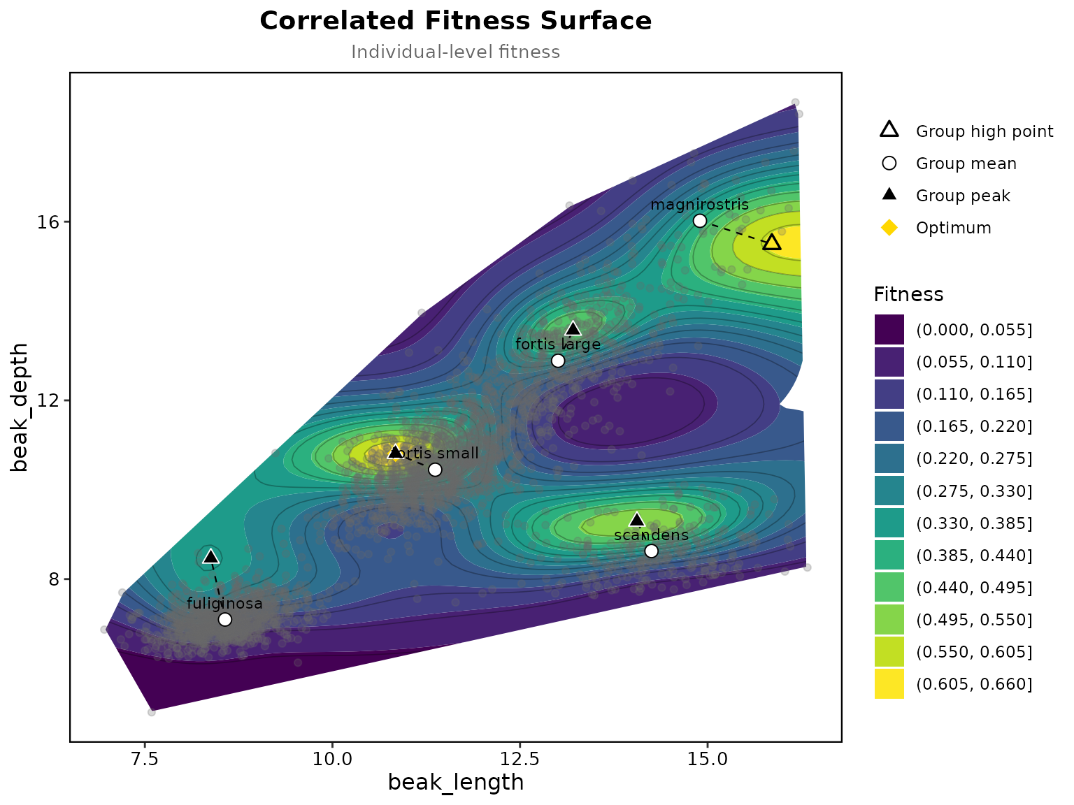
surface$groups## group n mean_beak_length mean_beak_depth peak_beak_length
## 1 fortis large 586 13.007307 12.886966 13.206667
## 2 fortis small 1384 11.369052 10.448229 10.840505
## 3 fuliginosa 1096 8.568677 7.095934 8.379697
## 4 magnirostris 53 14.897689 16.019465 15.856768
## 5 scandens 309 14.251929 8.627551 14.058485
## peak_beak_depth peak_fit peak_interior peak_edge
## 1 13.568485 0.4976503 TRUE FALSE
## 2 10.810909 0.6544065 TRUE FALSE
## 3 8.466970 0.3525709 TRUE FALSE
## 4 15.498788 0.6121519 FALSE FALSE
## 5 9.294242 0.5464443 TRUE FALSEGroup means lie 0.64 to 1.38 mm from the highest fitted lifespan in their range, 0.90 mm on average, as in Beausoleil et al. For fortis small, fortis large and scandens the distances match theirs within 0.03 mm. For fuliginosa ours is about a quarter of a millimetre shorter because they placed every peak within a rectangle drawn by hand. Their own model with the rule used here gives 1.42 mm. For magnirostris ours is about a quarter of a millimetre longer, and their model with our rule gives 0.88 mm, so there the fit differs. The flags say whether each high point is a peak: four groups sit by a peak of their own, and for magnirostris the surface keeps rising past its 53 birds towards the edge of the data. Every maximum of the surface is listed in the result.
surface$peaks## beak_length beak_depth fit interior
## 1 10.840505 10.810909 0.6544065 TRUE
## 2 16.235354 15.498788 0.6252551 FALSE
## 3 14.058485 9.294242 0.5464443 TRUE
## 4 13.206667 13.568485 0.4976503 TRUE
## 5 8.379697 8.466970 0.3525709 TRUEOverdispersion and the peak comparisons
The lifespans are overdispersed and the Poisson fit warns. With a
dispersion over three, Poisson standard errors are too small.
count_family = "quasipoisson" estimates the dispersion and
peak_difference() uses it in its standard errors. The
smoothness is chosen again under the new family, which moves the fitted
lifespan by a median of 0.01 years and by up to 41% of the Poisson value
in places.
surface$dispersion## [1] 3.359152
quasi <- correlated_fitness_surface(finches, "lifespan", c("beak_length", "beak_depth"),
                                    k = 27, too_far = 0.15, grid_n = 100, group = "species",
                                    group_effect = FALSE, count_family = "quasipoisson")
peak_difference(quasi, "fortis small", "fortis large", valley = TRUE)
## comparison fit_a fit_b difference se
## 1 fortis small - fortis large 0.6400272 0.4751763 0.2978247 0.3034674
## 2 fortis small - valley 0.6400272 0.2608015 0.8977511 0.3597152
## 3 fortis large - valley 0.4751763 0.2608015 0.5999264 0.4014420
## z p_value
## 1 0.9814061 0.3263925
## 2 2.4957275 NA
## 3 1.4944286 NA
peak_difference(quasi, "fortis small", "scandens", valley = TRUE)## comparison fit_a fit_b difference se z
## 1 fortis small - scandens 0.6400272 0.5156610 0.2160611 0.3740928 0.5775601
## 2 fortis small - valley 0.6400272 0.2914154 0.7867610 0.3280516 2.3982847
## 3 scandens - valley 0.5156610 0.2914154 0.5706999 0.4091962 1.3946854
## p_value
## 1 0.5635611
## 2 NA
## 3 NA
peak_difference(quasi, "fortis large", "scandens", valley = TRUE)## comparison fit_a fit_b difference se z
## 1 fortis large - scandens 0.4751763 0.5156610 -0.08176363 0.4070918 -0.2008482
## 2 fortis large - valley 0.4751763 0.2608015 0.59992635 0.4014420 1.4944286
## 3 scandens - valley 0.5156610 0.2608015 0.68168999 0.4424737 1.5406339
## p_value
## 1 0.8408173
## 2 NA
## 3 NA
peak_difference(quasi, "fortis large", "scandens", valley = TRUE, route = "line")## comparison fit_a fit_b difference se z
## 1 fortis large - scandens 0.4751763 0.51566103 -0.08176363 0.4070918 -0.2008482
## 2 fortis large - valley 0.4751763 0.08772981 1.68942425 0.6495500 2.6009151
## 3 scandens - valley 0.5156610 0.08772981 1.77118789 0.6285597 2.8178516
## p_value
## 1 0.8408173
## 2 NA
## 3 NAThe valley in each comparison is the pass, the lowest point on the
highest route between two high points. Fortis small sits about 2.5
standard errors above its passes to fortis large and to scandens, and
the lower of each pair about 1.5. Those z values run high (see
?peak_difference), so no pair is clearly separated, and no
high point is reliably higher than another. The straight line from
fortis large to scandens crosses a low patch at about 13.6 by 11.6 mm.
The route between them goes round it, past fortis small, so measuring
the valley on the line, as route = "line" does, makes the
two look far more separate than they are. The fuliginosa high point is
not an interior peak on this fit.
Checks on the peaks
Lifespan depends on when a bird was first caught, and the groups were caught at different times.
## 2003 2004 2005 2006 2007 2008 2009 2010 2011 2012 2013 2014 2015 2016 2017 2018
## 1.37 0.93 0.58 0.62 0.67 0.77 0.92 0.30 0.20 0.16 0.15 0.45 0.04 0.09 0.19 0.07
## 2019 2020
## 0.05 0.00
round(100 * prop.table(table(finches$species, cut(finches$first_year, c(2002, 2008, 2014, 2020),
                                                   labels = c("2003-08", "2009-14", "2015-20"))), 1))
##
## 2003-08 2009-14 2015-20
## fortis large 26 38 35
## fortis small 23 43 34
## fuliginosa 2 62 36
## magnirostris 42 45 13
## scandens 6 50 44Birds first caught in 2003 had an apparent lifespan of 1.4 years on average; those first caught in 2020 could not be seen again. Only 2% of the fuliginosa were first caught before 2009, against 42% of the magnirostris. On the birds first caught before 2020, models with the beak alone, the capture year alone and both show how much each accounts for:
d <- finches[finches$first_year < 2020, ]
d$first_year <- factor(d$first_year)
beak <- correlated_fitness_surface(d, "lifespan", c("beak_length", "beak_depth"),
                                   k = 27, too_far = 0.15, grid_n = 100, count_family = "quasipoisson")
year <- mgcv::gam(lifespan ~ first_year, family = quasipoisson(), data = d)
by_year <- correlated_fitness_surface(d, "lifespan", c("beak_length", "beak_depth"),
                                      k = 27, too_far = 0.15, grid_n = 100, group = "first_year",
                                      count_family = "quasipoisson")
explained <- round(100 * c(beak = summary(beak$model)$dev.expl, year = summary(year)$dev.expl,
                           both = summary(by_year$model)$dev.expl))
explained
## beak year both
## 5 16 18
at <- function(g) unlist(quasi$groups[quasi$groups$group == g, c("peak_beak_length", "peak_beak_depth")])
peak_difference(by_year, at("fortis small"), at("fortis large"), valley = TRUE)
## comparison fit_a fit_b difference se
## 1 (10.8, 10.8) - (13.1, 13.6) 0.1952896 0.1675461 0.1532248 0.2687174
## 2 (10.8, 10.8) - valley 0.1952896 0.1381010 0.3464980 0.6618802
## 3 (13.1, 13.6) - valley 0.1675461 0.1381010 0.1932732 0.7088948
## z p_value
## 1 0.5702079 0.5685367
## 2 0.5235056 NA
## 3 0.2726402 NA
peak_difference(by_year, at("fortis large"), at("scandens"), valley = TRUE)## comparison fit_a fit_b difference se
## 1 (13.1, 13.6) - (14.2, 9.29) 0.1675461 0.2366871 -0.3454801 0.3507725
## 2 (13.1, 13.6) - valley 0.1675461 0.1381010 0.1932732 0.7088948
## 3 (14.2, 9.29) - valley 0.2366871 0.1381010 0.5387534 0.6812626
## z p_value
## 1 -0.9849123 0.3246672
## 2 0.2726402 NA
## 3 0.7908159 NAOn the same birds the year of first capture alone explains 16% of the deviance, beak length and depth 5%, and the two together 18%. With the year in the model, at the same high points the passes are shallow, with no pair well above the valley between them. The peaks also depend on the fit. With a smaller basis, or a negative binomial family, only scandens keeps a peak of its own:
k20 <- correlated_fitness_surface(finches, "lifespan", c("beak_length", "beak_depth"),
                                  k = 20, too_far = 0.15, grid_n = 100, group = "species",
                                  group_effect = FALSE, count_family = "quasipoisson")
nb <- correlated_fitness_surface(finches, "lifespan", c("beak_length", "beak_depth"),
                                 k = 27, too_far = 0.15, grid_n = 100, group = "species",
                                 group_effect = FALSE, count_family = "nb")
data.frame(group = quasi$groups$group, k27 = quasi$groups$peak_interior,
           k20 = k20$groups$peak_interior, nb = nb$groups$peak_interior)
## group k27 k20 nb
## 1 fortis large TRUE FALSE FALSE
## 2 fortis small TRUE FALSE FALSE
## 3 fuliginosa FALSE FALSE FALSE
## 4 magnirostris FALSE FALSE FALSE
## 5 scandens TRUE TRUE TRUEThe same surface on standardised traits
The usual route in the package standardises the traits first. The peaks come back in millimetres by undoing the scaling.
prep <- prepare_selection_data(finches, "lifespan", c("beak_length", "beak_depth"))
surface_z <- correlated_fitness_surface(prep, "lifespan", c("beak_length", "beak_depth"),
                                        k = 27, too_far = 0.15, group = "species", group_effect = FALSE)
g <- surface_z$groups
sds <- sapply(finches[, c("beak_length", "beak_depth")], sd)
mus <- colMeans(finches[, c("beak_length", "beak_depth")])
g$peak_length_mm <- g$peak_beak_length * sds[1] + mus[1]
g$peak_depth_mm <- g$peak_beak_depth * sds[2] + mus[2]
g[, c("group", "n", "peak_length_mm", "peak_depth_mm")]
## group n peak_length_mm peak_depth_mm
## 1 fortis large 586 13.153729 13.580169
## 2 fortis small 1384 10.771525 10.803898
## 3 fuliginosa 1096 8.389322 8.490339
## 4 magnirostris 53 15.853559 15.662373
## 5 scandens 309 14.265424 9.415763