Fitness functions and adaptive landscapes over time
Source:R/temporal_landscape.R
temporal_landscape.RdFits the fitness function (one trait) or fitness surface (two traits) separately for each level of a time column, usually year, and optionally the adaptive landscape for each, to show how selection changes over time. Beausoleil et al. (2019) did this for Darwin's finches, one year at a time.
Usage
temporal_landscape(
  data,
  fitness_col,
  trait_cols,
  time_col,
  fitness_type = c("auto", "binary", "count", "continuous"),
  min_n = 20,
  landscape = TRUE,
  k = NULL,
  bs = NULL,
  smoothing = NULL,
  bootstrap = FALSE,
  n_boot = 200,
  grid_n = 60,
  simulation_n = 300,
  mask = TRUE,
  too_far = NULL,
  count_family = c("poisson", "quasipoisson", "nb")
)
Arguments
- data
A data frame with fitness, trait and time columns. Standardise the traits once, over all periods, with
prepare_selection_data()before calling; the periods must share one trait axis, so nothing is restandardised per period.- fitness_col
Name of the fitness column.
- trait_cols
One or two trait column names.
- time_col
Name of the column giving the period of each row.
- fitness_type
Passed to
univariate_spline()for one trait; the surface detects the type itself.- min_n
Periods with fewer complete rows than this are skipped and listed in the result's
skipped. Default is 20.- landscape
Logical; also compute the adaptive landscape for each period. Default is
TRUE.- k, bs, smoothing
Basis size, basis and smoothing criterion for the period fits.
NULLuses the defaults ofunivariate_spline()orcorrelated_fitness_surface().- bootstrap, n_boot
For one trait, a bootstrap band around each period's fitness function.
- grid_n
Grid resolution for the surfaces and landscapes.
- simulation_n
Simulated individuals per grid point in the landscapes.
- mask, too_far
Passed to
correlated_fitness_surface()for two traits.- count_family
Family for count fitness in every period's fit:
"poisson"(the default),"quasipoisson"or"nb", as inunivariate_spline().
Value
An object of class "temporal_landscape": fits and
landscapes, one per period; summary, one row per period
with n, mean fitness, trait means, the smooth's degrees of freedom, the
position and height of the highest fitted fitness and whether it sits at
the edge of the data (optimum_edge), the number of interior
peaks (one trait) and the landscape optimum; grid, the fitted
values of every period stacked with a time column; for one trait
heat, each period's fitness function on one common trait grid,
NA outside that period's data; landscape_grid, the
landscapes stacked; data, the rows used; and skipped.
Examples
prep <- prepare_selection_data(finch_yearly, "survived", "beak_pc1")
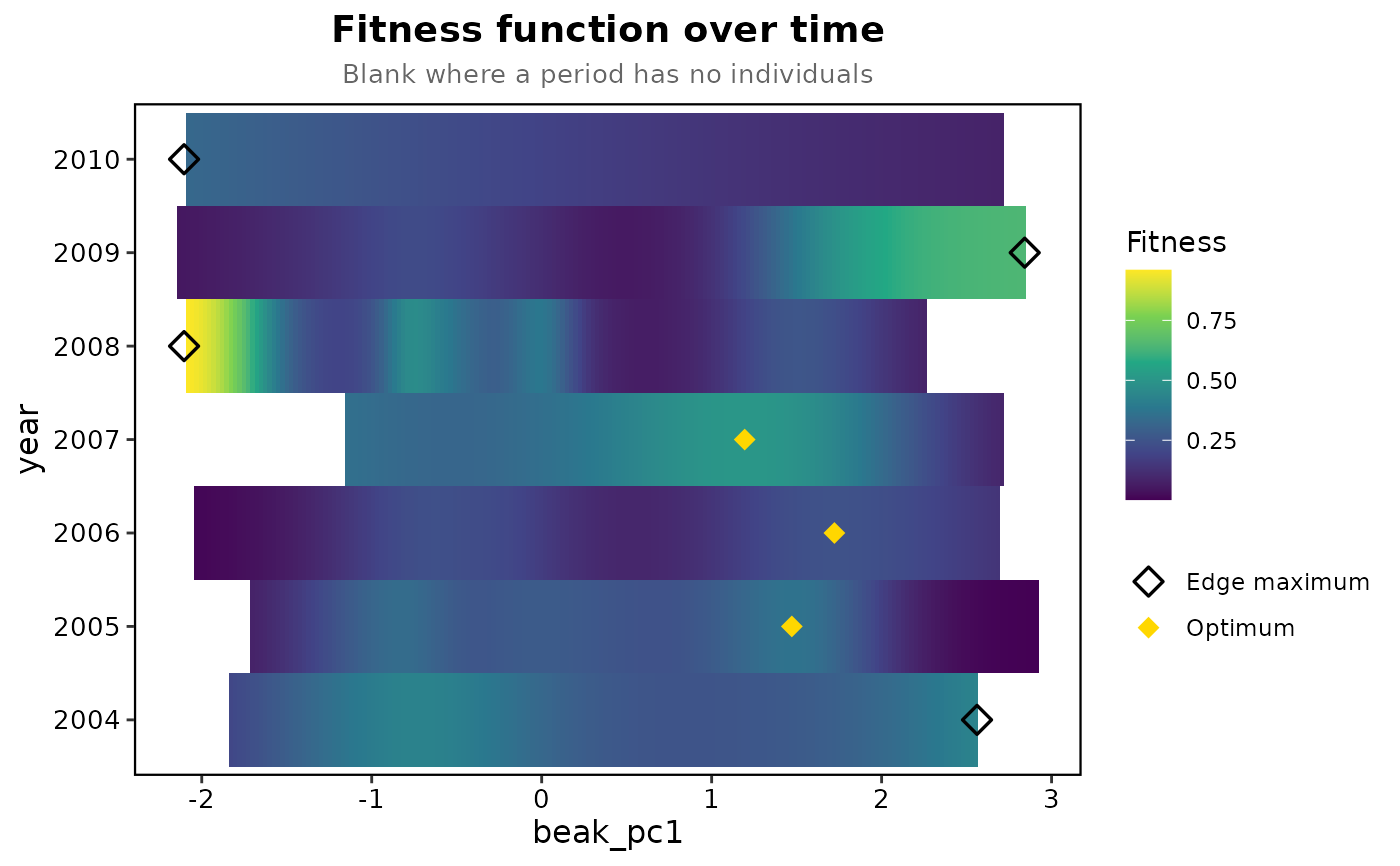
years <- temporal_landscape(prep, "survived", "beak_pc1", "year", landscape = FALSE)
#> 2004: n = 110, mean fitness 0.345, edf 3.0, 1 interior peak, highest fitness at the edge of the data
#> 2005: n = 185, mean fitness 0.276, edf 5.2, 3 interior peaks
#> 2006: n = 233, mean fitness 0.180, edf 4.4, 2 interior peaks
#> 2007: n = 61, mean fitness 0.344, edf 2.7, 1 interior peak
#> 2008: n = 127, mean fitness 0.307, edf 7.0, 3 interior peaks, highest fitness at the edge of the data
#> 2009: n = 196, mean fitness 0.194, edf 4.8, 1 interior peak, highest fitness at the edge of the data
#> 2010: n = 175, mean fitness 0.189, edf 1.0, 0 interior peaks, highest fitness at the edge of the data
years$summary
#>   time   n mean_fitness mean_beak_pc1      edf optimum_beak_pc1 optimum_fit
#> 1 2004 110    0.3454545    0.15262095 3.039609         2.561262   0.4325621
#> 2 2005 185    0.2756757    0.01659862 5.210404         1.471795   0.3642465
#> 3 2006 233    0.1802575   -0.07931978 4.447501         1.722241   0.2434433
#> 4 2007  61    0.3442623    0.12403720 2.732732         1.194424   0.5077420
#> 5 2008 127    0.3070866   -0.12870140 6.962240        -2.103969   0.9659317
#> 6 2009 196    0.1938776   -0.08518852 4.813914         2.841979   0.6449075
#> 7 2010 175    0.1885714    0.13770410 1.000049        -2.103969   0.3286811
#>   optimum_edge peaks
#> 1         TRUE     1
#> 2        FALSE     3
#> 3        FALSE     2
#> 4        FALSE     1
#> 5         TRUE     3
#> 6         TRUE     1
#> 7         TRUE     0
plot_temporal_landscape(years, type = "heatmap")