Plot Fitness Surfaces Comparison

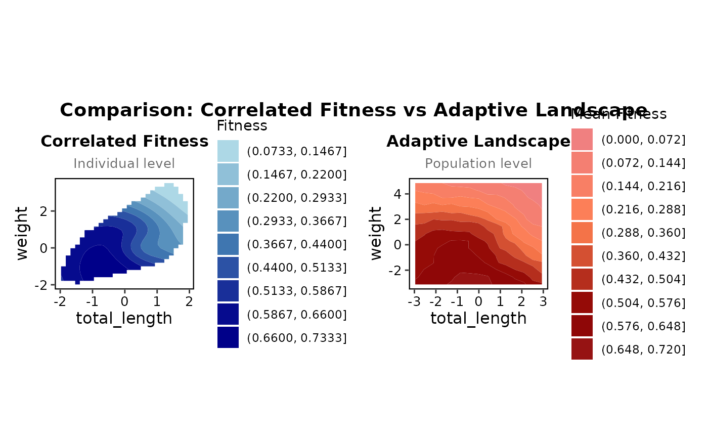
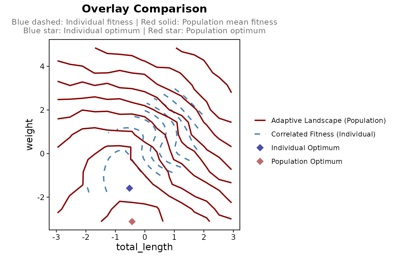
Visualizes the comparison between individual-level correlated fitness and population-level adaptive landscape.

Usage

plot_fitness_surfaces_comparison(
  comparison_data,
  bins = 10,
  title = NULL,
  point_alpha = 0.7,
  linewidth = 0.8,
  show_optima = TRUE
)

Arguments

comparison_data

Output list from compare_fitness_surfaces_data().

bins

Integer specifying the number of contour bins. Default is 10.

title

Optional character string for the overarching plot title.

point_alpha

Numeric value for optimum point transparency. Default is 0.7.

linewidth

Numeric value for contour line width. Default is 0.8.

show_optima

Logical indicating whether to show optimum points on the overlay. Default is TRUE.

Value

A list containing side_by_side (a patchwork object) and overlay (a ggplot object).

Examples

prep <- prepare_selection_data(bumpus, "survival", c("total_length", "weight"))
surf <- correlated_fitness_surface(prep, "survival", c("total_length", "weight"), grid_n = 30)
#> Data type: binary; method: gam; n = 136; k = 29
#> GAM fitting with 136 observations
#>   Trying formula: main
#> Success with formula: main
#> Predictions range: 0.0472 to 0.703
#> Masked 424 of 900 grid points outside the data
land <- adaptive_landscape(prep, surf$model, c("total_length", "weight"),
                           simulation_n = 100, grid_n = 15)
#> Population mean grid ranges:
#>   total_length: -2.96 to 2.94
#>   weight: -3.12 to 4.85
#> Estimated within-population variance-covariance:
#>              total_length weight
#> total_length       1.0000 0.5839
#> weight             0.5839 1.0000
#> Calculating mean fitness for 225 grid points
#> Optimal population mean phenotype:
#>   total_length    weight
#> 7   -0.4336396 -3.121579
#> Mean fitness at optimum: 0.6738
#> The highest mean fitness is on the edge of the grid; the landscape may keep rising beyond it
#> 76% of simulated individuals fell outside the data (96% at the optimum)
#> The optimum rests on extrapolation: more than 25% of the population simulated there lies outside the data
comp <- compare_fitness_surfaces_data(surf, land, c("total_length", "weight"))
#> Warning: Grid sizes differ: correlated surface has 900 points, adaptive landscape has 225 points.
#> Comparison may be affected. Consider using same grid_n.
#> Individual optimum:
#>    total_length    weight   fitness
#> 72   -0.5207948 -1.590066 0.7030432
#> Population optimum:
#>   total_length    weight   fitness
#> 7   -0.4336396 -3.121579 0.6738219
#> Distance between optima: 1.534
#> Summary statistics:
#>              Surface Fitness_Range_Min Fitness_Range_Max Fitness_Mean
#> 1 Correlated Fitness        0.07483220         0.7030432    0.4668537
#> 2 Adaptive Landscape        0.02484124         0.6738219    0.3830345
#>   Fitness_SD N_Points
#> 1  0.1865585      900
#> 2  0.1910124      225
plot_fitness_surfaces_comparison(comp)
#> $side_by_side
#> Warning: Removed 424 rows containing non-finite outside the scale range
#> (`stat_contour_filled()`).

#> 
#> $overlay
#> Warning: Removed 424 rows containing non-finite outside the scale range
#> (`stat_contour()`).

#>